


DIY #5 - Set a benchmark for your model
DIY #5 - Set a benchmark for your model
Do It Yourself is part of Machine Learning Pills: mlpills.dev

💊 Pill of the week
In this issue, we will talk about base models for Time Series forecasting.
What are base models?
In Time Series Analysis and Forecasting, a base model is often a simple model used as a benchmark to compare the performance of more complex models. Here are several basic or naive methods that are commonly used as base models in time series forecasting:
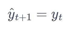
1. Naive Forecast (NF)
This method simply uses the last observed value as the forecast for all future time points. It is naive because it does not consider any other information from the past.
Formula:

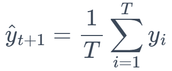
2. Simple Average (SA)
This method calculates the average of all past observations and uses this value as the forecast. It assumes that future values will revolve around the average of past values.
Formula:

where 𝑇 is the number of observations.
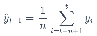
3. Moving Average (MA)
This method averages the last n observations to forecast the next value. It smoothens short-term fluctuations and highlights longer-term trends or cycles.
Formula:

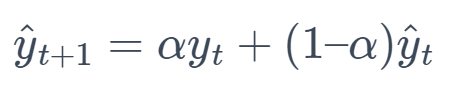
4. Exponential Smoothing (ES)
This method gives more weight to the most recent observations and less weight to the older ones, with weights decreasing exponentially.
Formula:

where α is the smoothing parameter.
Do you want to take your ML skills to the next level? Discover Train In Data:

Self-passed online learning courses, featuring in-depth modules on feature engineering and selection, working with imbalanced data, optimizing hyperparameters, time series forecasting and more. A great complement to MLPills to take your skills to the next level!
*Sponsored: by purchasing any of their courses you would also be supporting MLPills.
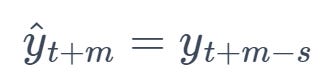
5. Seasonal Naive Forecast (SNF)
This method assumes that the future value will be equal to the last observed value from the same season.
Formula:

where s is the seasonal period and m is the forecast horizon.
6. Drift Method (DM)
This method extrapolates the line connecting the first and the last observation to forecast future values.
Formula:
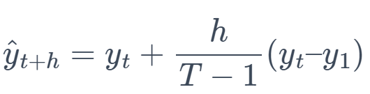
where h is the forecast horizon and T is the number of observations.

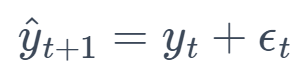
7. Random Walk (RW)
This method assumes that changes in the time series are random, and future values are unpredictable, being equal to the last observed value plus a random error.
Formula:

where ϵₜ is a white noise error term.
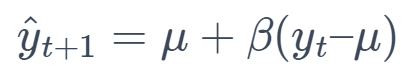
8. Mean Reversion (MR)
This method assumes that the series will revert to its mean over time, forecasting future values based on the mean and the last observed value.
Formula:

where μ is the mean and β is the reversion coefficient.
How to Choose a Base Model?
Simplicity: Base models are typically simple and easy to understand.
Data Characteristics: Consider the characteristics of the data, such as seasonality and trend, when choosing a base model.
Performance Metric: Evaluate the base model using appropriate performance metrics like MAE, RMSE, or MAPE to set a benchmark for more sophisticated models.
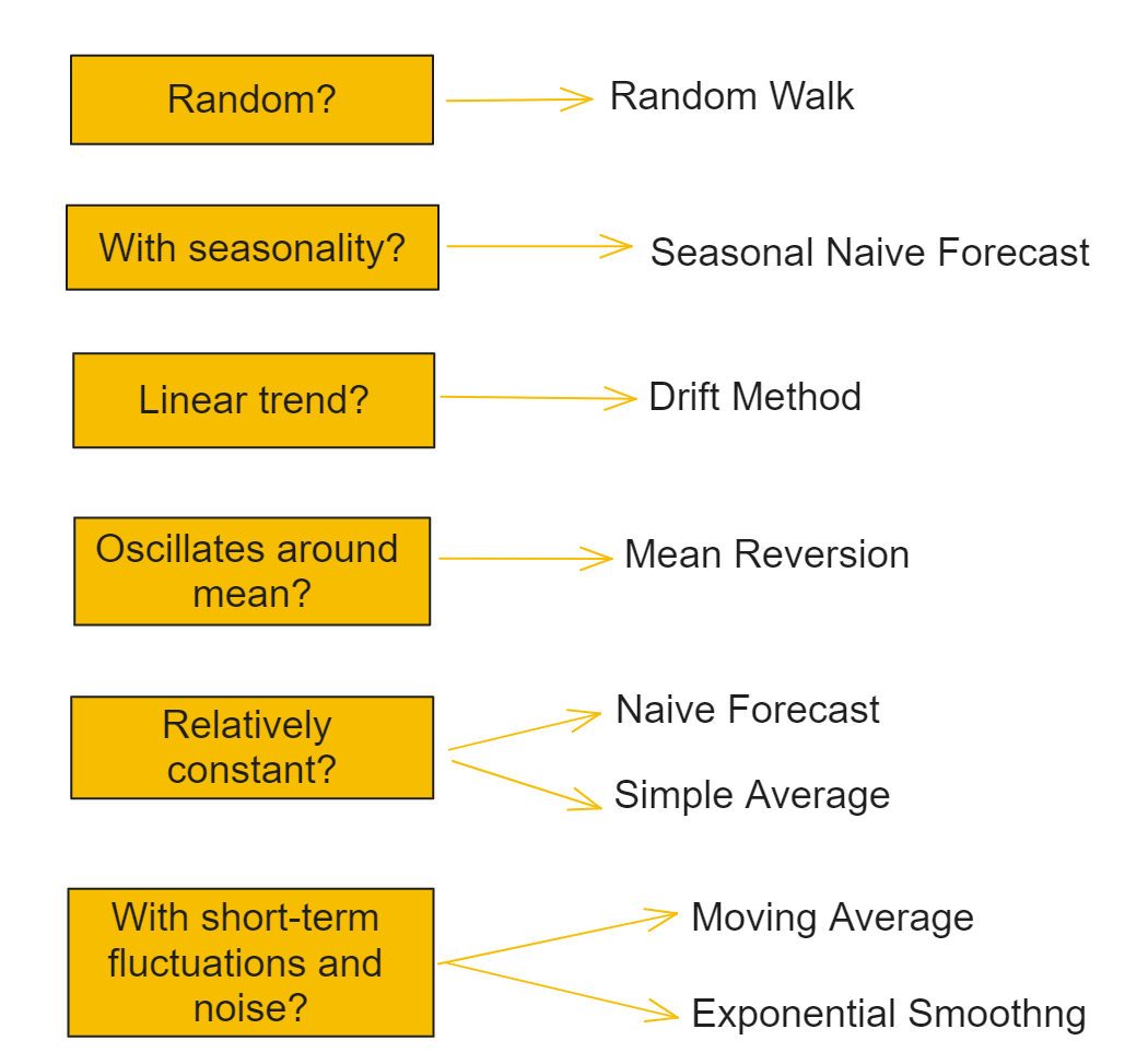
Here is a simple diagram to help you choose the best benchmark model. You could also select multiple ones and keep the one that shows a better performance.
Conclusion
These naive methods serve as a starting point and help in establishing a baseline performance. Any sophisticated model should ideally perform significantly better than these naive models to be considered useful.
👉 Check the next section to put what you've learned into practice!
This could perfectly be a Data Science interview question. You can check additional questions on the website!
If you like it, subscribe for free to support us:
🛠️ Do It Yourself!
Now that you know the theory about base models and when you should use each of them, it’s time to apply it!
How does it work?
📜I will share a notebook with some guided initial steps.
📌I will ask you some tasks that you should complete.
🎯I will share the outcome so you can check if you did well or not!
Now it’s your turn. Let’s play!
I want you to apply each of the five techniques I previously introduced:
🖨Naive Forecast - Difficulty ⭐
⚖️Simple Average - Difficulty ⭐
🪟Moving Average - Difficulty ⭐
🥑Exponential Smoothing - Difficulty ⭐⭐
🏖Seasonal Naive Forecast - Difficulty ⭐⭐
🛝Drift Method - Difficulty ⭐⭐
🎲Random Walk - Difficulty ⭐
🎢Mean Reversion - Difficulty ⭐
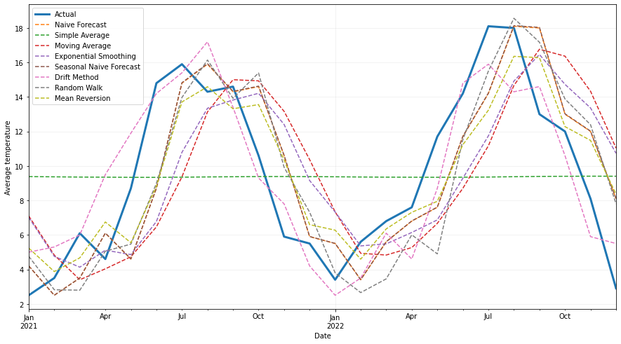
I provide you with the average monthly temperature in London for the last 40 years (1982 - 2022). Create eight base models to see which one behaves better when forecasting the last 2 years. You will then be able to use this model as the benchmark when you train a more complex model like SARIMA, Holt-Winters, LSTM…
You should get something like this:
Here you can find a Kaggle notebook with everything you need below:
Keep reading with a 7-day free trial
Subscribe to Machine Learning Pills to keep reading this post and get 7 days of free access to the full post archives.