

Issue #137 - From Randomized to Natural Experiments

💊 Pill of the Week
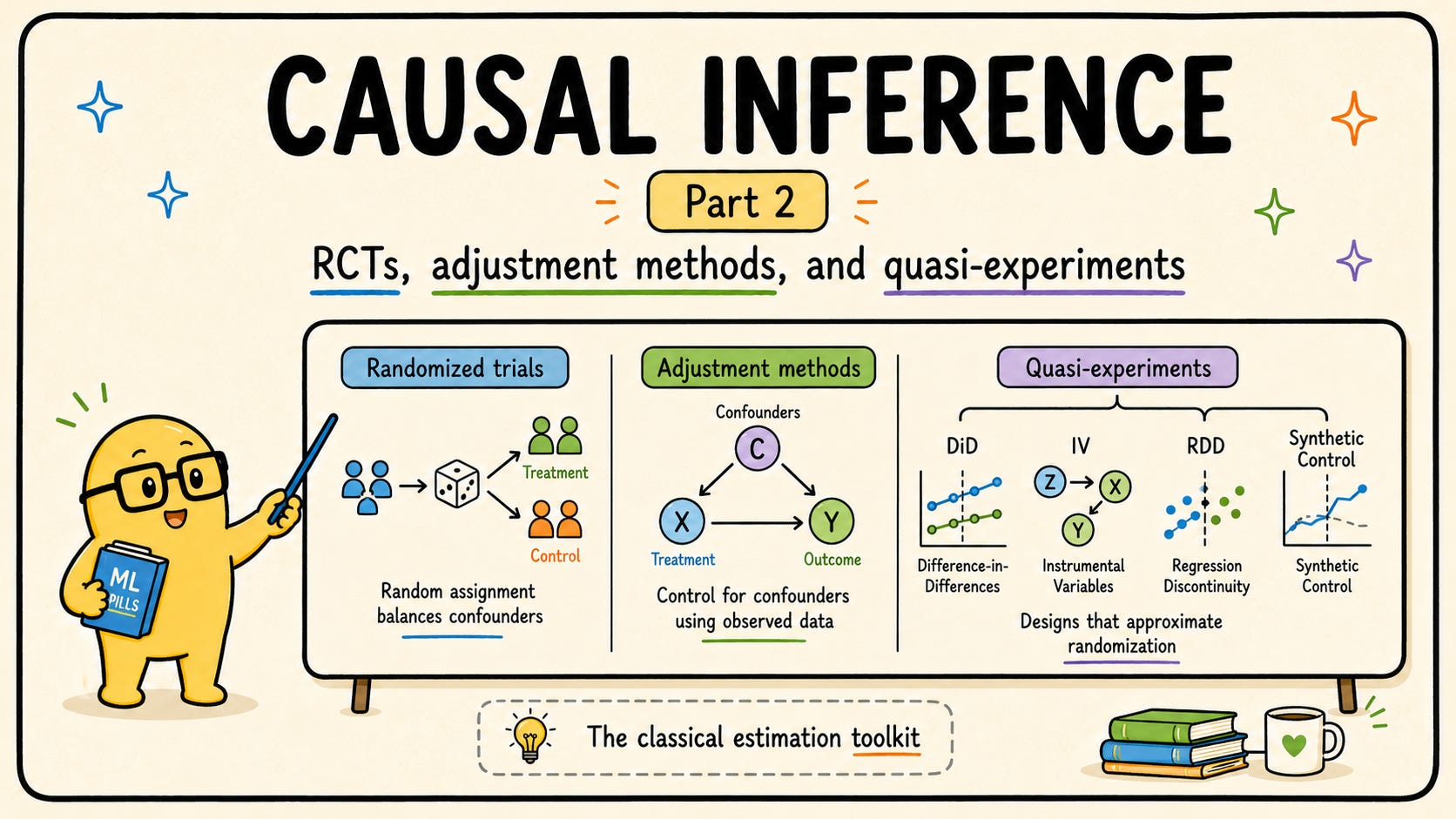
In Part 1 we established the problem: causal effects are defined by counterfactuals, and counterfactuals are never observed. We also covered the two frameworks (potential outcomes and DAGs) that tell us what to estimate and which assumptions we need.

This issue is about the how. We will walk through the classical estimation toolkit in increasing order of desperation, moving from the gold standard of randomization, to adjustment methods for when you have measured the confounders, and finally to quasi-experimental designs for when you have not but nature has been kind to you.
Part 1: foundations, frameworks, and the fundamental problem.
Part 2 (this issue): RCTs, adjustment-based methods, and quasi-experimental designs.
Part 3: ML-based causal inference, uplift modeling, and tooling.
Randomized Controlled Trials: The Gold Standard
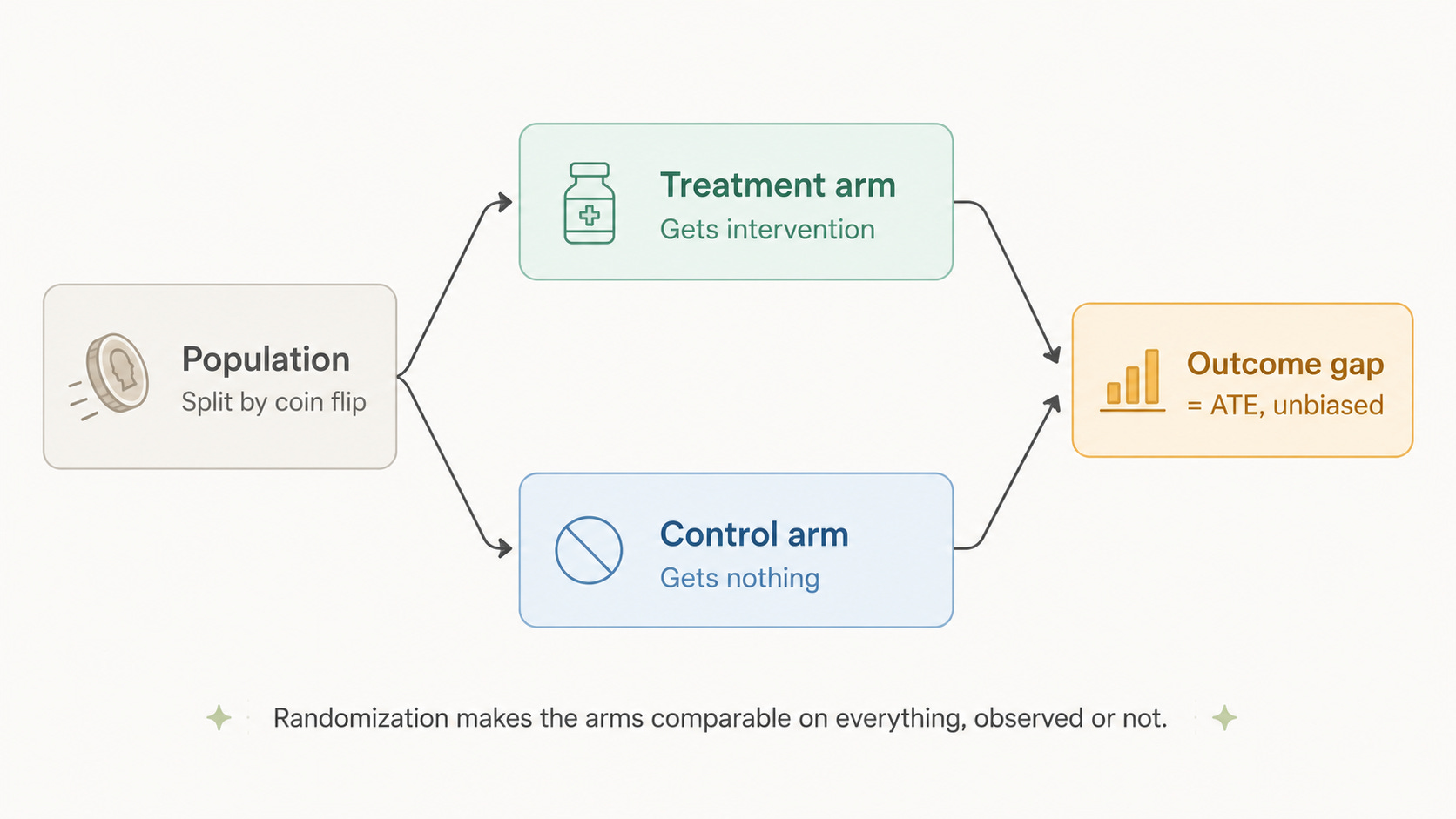
Randomization solves the identification problem by brute force. If treatment is assigned by coin flip, assignment cannot be correlated with anything, observed or unobserved, so the treated and control groups become statistically exchangeable and a simple difference in means is an unbiased estimate of the ATE. That single property is why the RCT is the reference standard across every field that can afford one, from clinical trials for drug approval, to A/B tests for features and pricing, to the development-economics RCT movement that tests interventions like deworming programs and cash transfers.
The trouble is that experiments are frequently off the table. Sometimes randomizing is unethical, as with assigning people to smoke for twenty years. Sometimes it is infeasible, as with randomizing interest rates by customer in a regulated market or randomizing a nationwide law. Sometimes the treatment is simply not under your control, like a competitor’s price move or a pandemic. And sometimes it is just too slow or too expensive, because the effect takes years to materialize or exposing half your traffic to a risky variant costs too much. Everything else in this article exists precisely for those cases.
Adjustment-Based Methods
Adjustment methods all lean on the same strong assumption: unconfoundedness, meaning you have measured every confounder X. Granting that, the entire game reduces to comparing treated and untreated units that share the same X. They differ only in how they carry out that comparison.
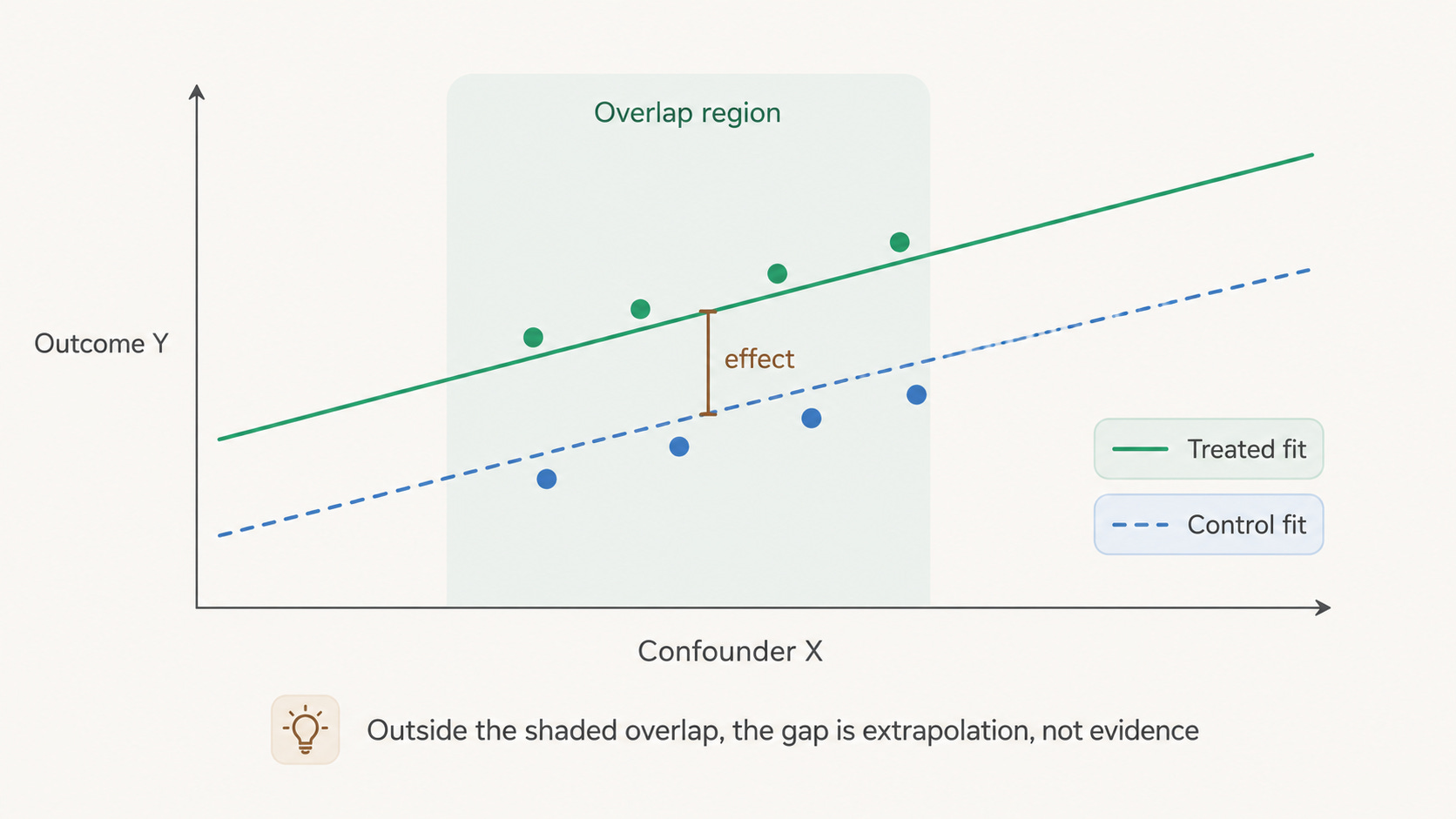
The most familiar approach is regression adjustment, where you model the outcome as a function of treatment and confounders and read the effect off the treatment term, or equivalently take the difference of predictions under T=1 and T=0. It is simple and it is everywhere, but it is fragile to model misspecification and it will cheerfully extrapolate into regions where treated and control units do not overlap, manufacturing counterfactuals out of thin air.
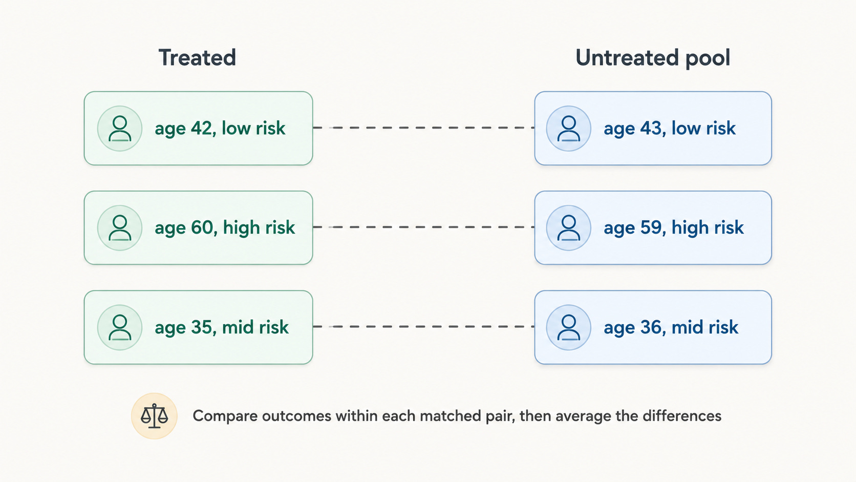
Matching tackles the comparison more directly by pairing each treated unit with one or more untreated units that have similar covariates, then contrasting outcomes within each pair. A hospital study, for instance, might pair each treated patient with an untreated patient of the same age, sex, and comorbidity profile. It is intuitive and transparent, but exact matching collapses under the curse of dimensionality as the covariate count grows.
Propensity scores rescue matching from that collapse. You do not need to match on all of X, only on a single number: the propensity score e(X) = P(T = 1 | X), the probability of receiving treatment given covariates. You estimate it with any classifier and then put it to work in one of three ways:
Matching treated and control units that have similar scores.
Stratifying the sample into propensity bins and averaging the within-bin contrasts.
Weighting each unit by the inverse of its assignment probability (IPW), which builds a pseudo-population in which treatment is independent of X.
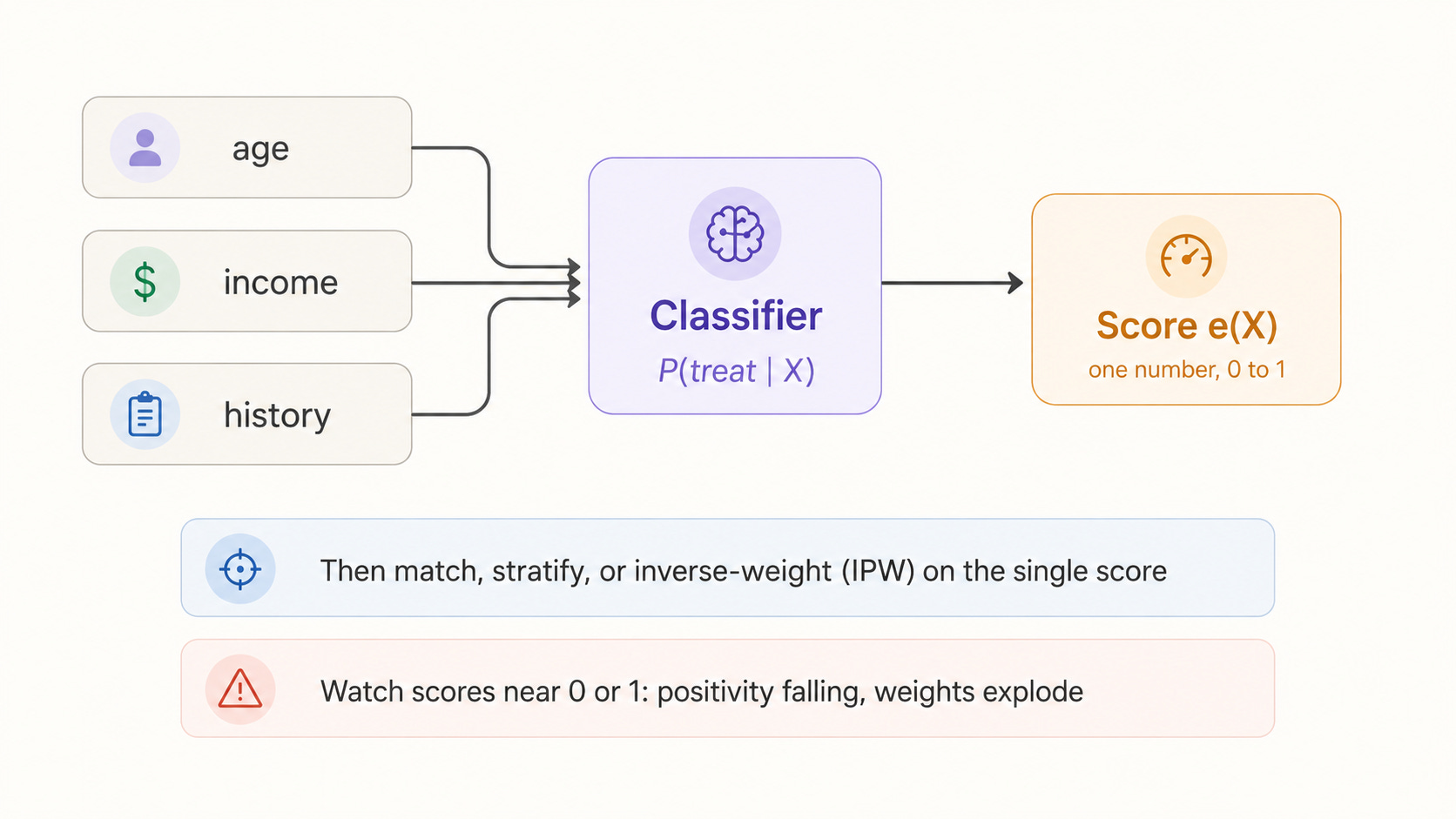
Two practical warnings travel with propensity methods. Check the overlap of the propensity distributions, because scores bunched near 0 or 1 are a sign that positivity is failing, and watch for exploding IPW weights, which trimming or stabilized weights will tame.
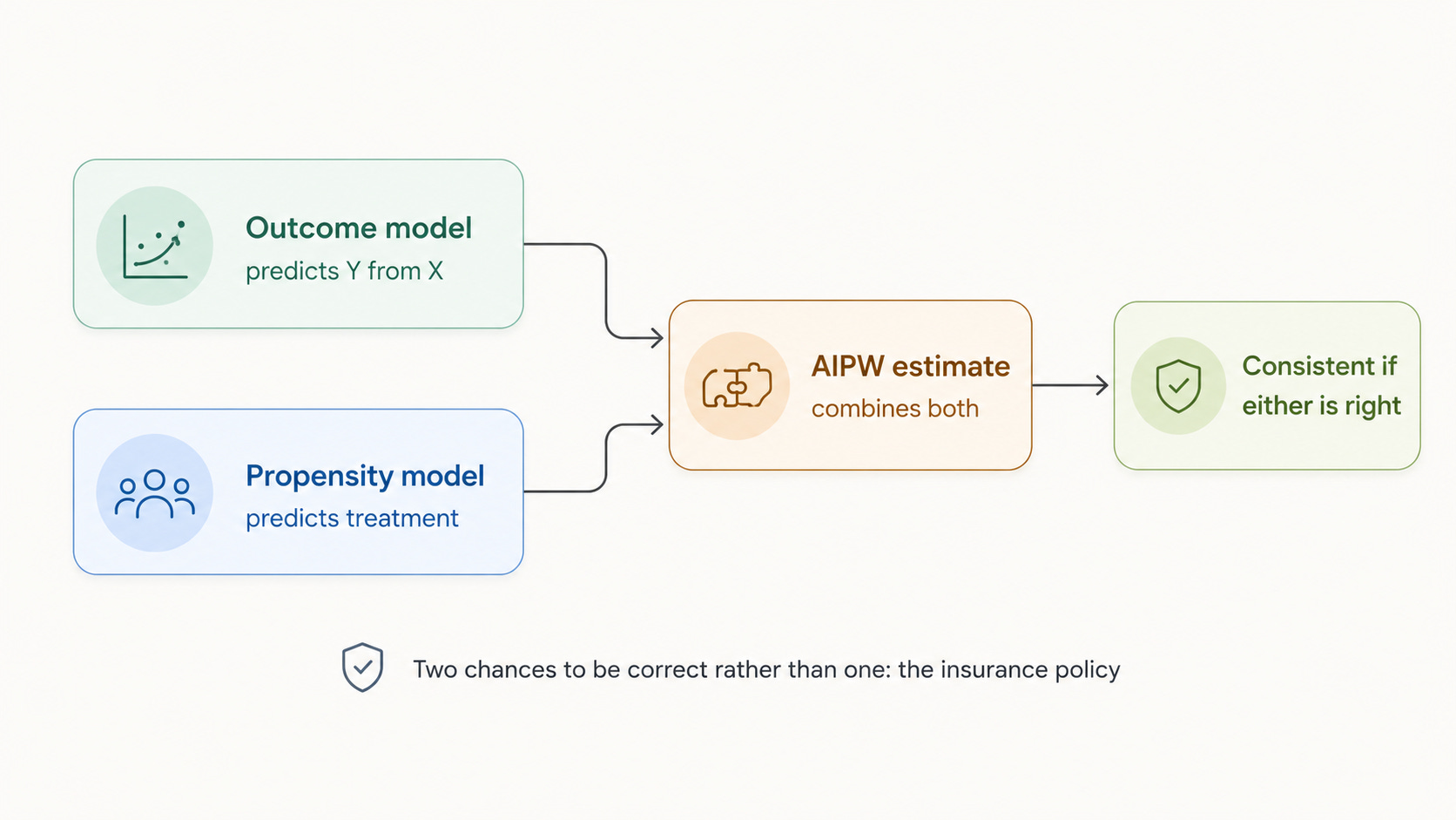
Finally, doubly robust estimation (AIPW) combines an outcome model and a propensity model into a single estimator that stays consistent if either one is correctly specified. Given that both models are usually a little wrong, that is a genuinely valuable insurance policy, and it is exactly this idea, made compatible with flexible ML, that becomes Double Machine Learning in Part 3.
Quasi-Experimental Methods
Adjustment methods die the moment an important confounder goes unmeasured. Quasi-experimental designs get around that by exploiting natural experiments, situations where some quirk of policy, geography, timing, or a threshold rule assigns treatment in a way that is plausibly unrelated to the unmeasured confounders. The four workhorses below each exploit a different kind of quirk.
1. Difference-in-Differences (DiD)
DiD compares the before-and-after change in a treated group against the before-and-after change in an untreated group, and that second difference nets out both fixed differences between the groups and any trend they share over time. The canonical case is Card and Krueger’s minimum wage study, where New Jersey raised its minimum wage and neighboring Pennsylvania did not; comparing the change in fast-food employment across the two states isolates the policy effect. The design rests on the parallel trends assumption, that absent the treatment both groups would have evolved the same way.
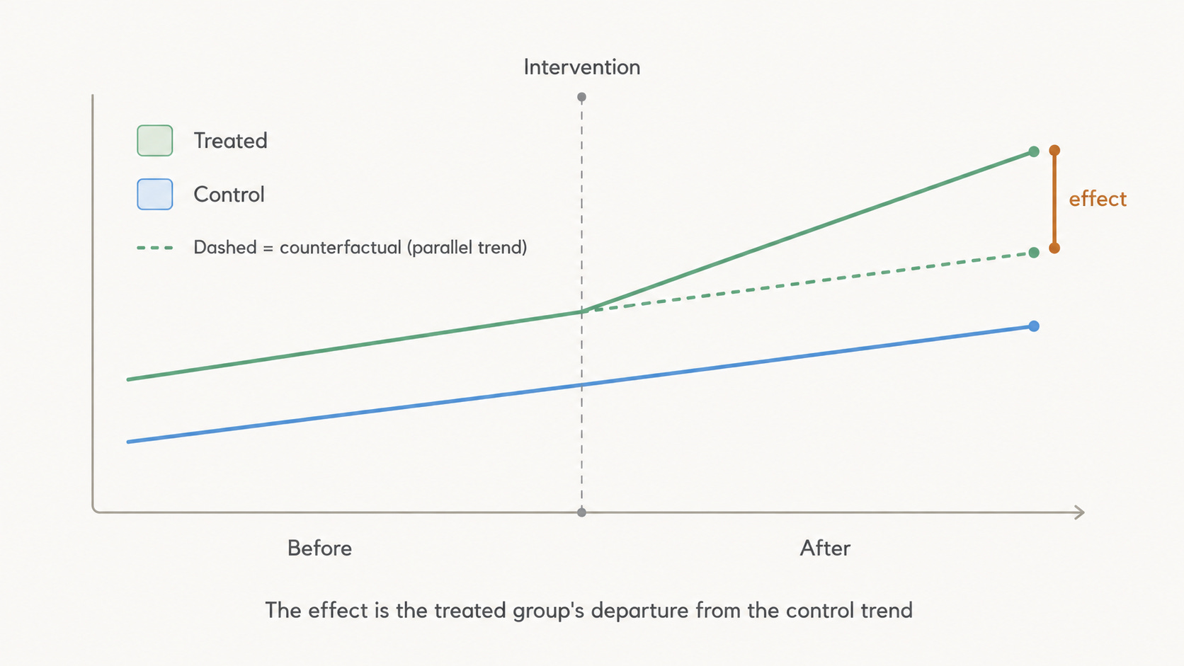
Industry versions of this are everywhere, whether a feature rolled out to some markets first, a policy applied to one customer segment, or a price update shipped to some regions. The one discipline that matters is to plot the pre-treatment trends for both groups, because if they were not parallel before the intervention, the whole design is already in trouble.
🔒 The rest of this section is for paid subscribers
💎Please become a paid subscriber to unlock the other methods, as this is exclusive content for paid subscribers💎
Choosing a Method: A Rough Decision Guide
The methods above line up naturally as a sequence of fallbacks, each one for the case where the previous option is unavailable:
Can you randomize? Do it. Even a small holdout beats a large observational analysis.
All confounders measured, with decent overlap? Reach for adjustment methods, ideally a doubly robust estimator rather than propensity scores alone.
Unmeasured confounding, but a policy or rollout with before-and-after data? Use DiD if you have a control group (and check parallel trends), or synthetic control if only one unit is treated.
A threshold rule assigns treatment? RDD.
A plausible instrument exists? IV, held to a high bar of skepticism.
None of the above? Then the honest answer may be that the effect is not identifiable from your data, and the real deliverable is a designed experiment rather than an estimate.
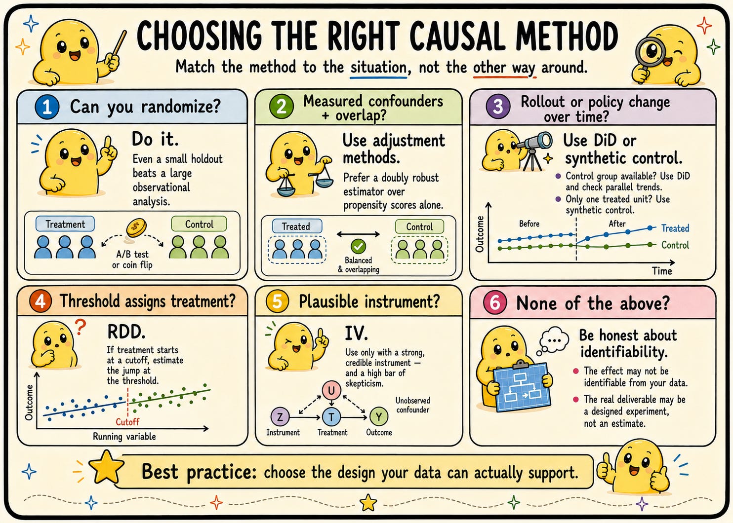
Whatever you land on, estimate with more than one method when you can. Agreement across designs that rest on different assumptions is the closest observational work ever gets to proof.
Coming Up in Part 3…
Classical methods mostly target the average effect, but averages hide the structure that actually drives decisions: a drug that helps some patients and harms others, a campaign that persuades some customers and annoys the rest.
Part 3 turns to the ML side of causal inference, where we estimate heterogeneous effects at the individual level through meta-learners, Double Machine Learning, causal forests, and uplift modeling, together with the libraries (DoWhy, EconML, CausalML) that put all of it within a pip install.
Thanks!