Issue #138 - A Field Guide to Tree Models

Jul 30, 2026

💊 Pill of the Week

Almost every tabular problem you will ever ship is solved by a tree. Not a neural network, not a linear model. A tree, or a few hundred of them stacked in some clever way.

The confusing part is that “tree model” covers a dozen different algorithms with genuinely different behaviour, and the names do not tell you much. This is a tour of the ones worth knowing. For each one: what it is, how it actually works, three lines to train it, and the one property that makes it different from its neighbours.

Paid subscribers get one extra:

The companion 💎Jupyter Notebook💎 with all the code plus additional analysis and visualisations, going out next Monday!

⚠️After that date it’s gone for anyone not already subscribed.

Don’t miss it!

What every tree has in common

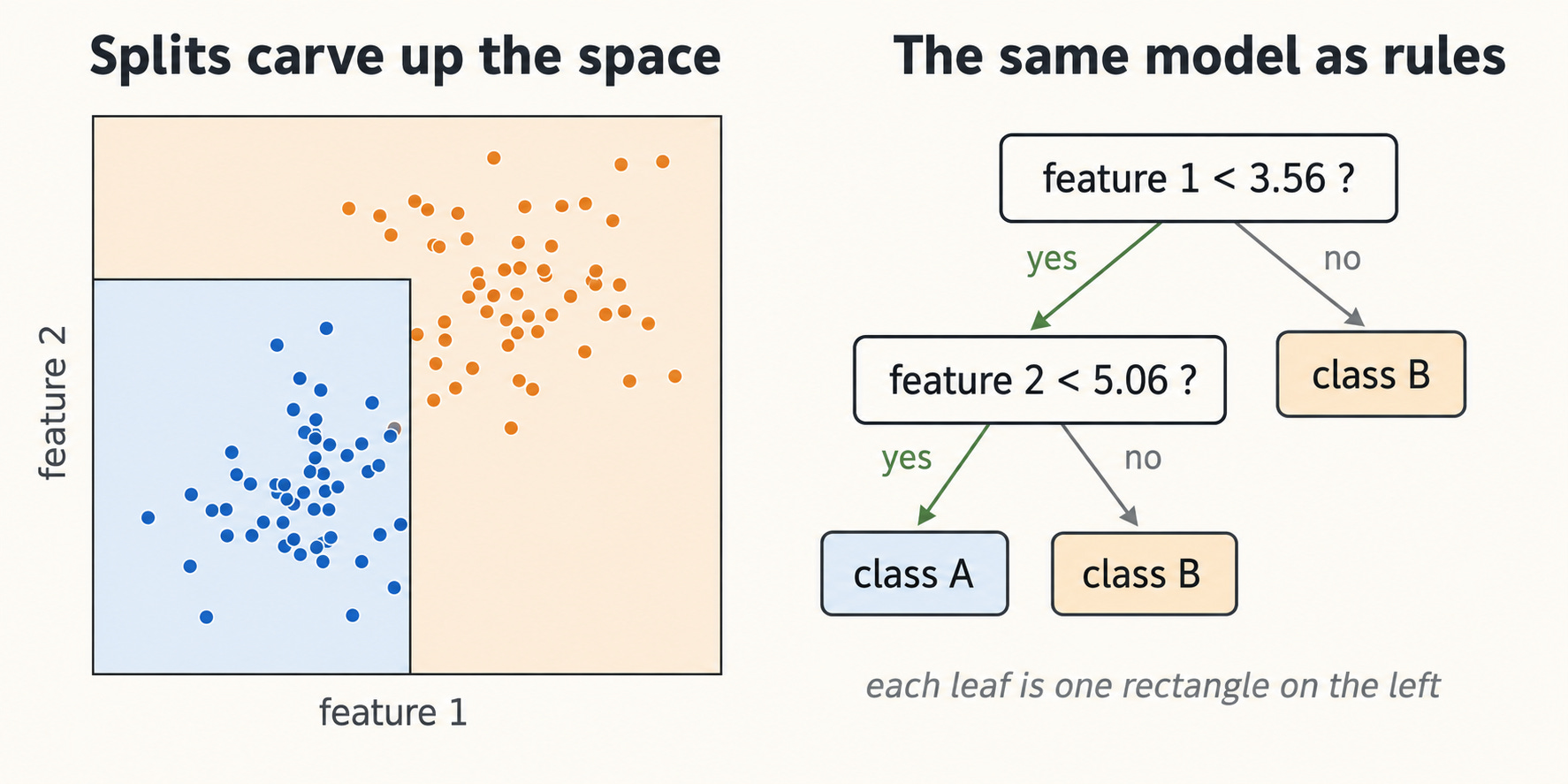
Before the differences, the shared machinery. Every model here does the same basic thing: it slices the feature space into boxes with cuts that are perpendicular to the axes, and predicts a single constant inside each box.

That one design choice explains most of the practical behaviour.

Scaling a feature does nothing. A split is a question about ordering (”is age below 40”), so any monotone transform of a feature leaves the tree unchanged. Standardising, taking logs, converting to ranks: same tree, same predictions. This is why tree models need so little preprocessing.
Mixed data is fine. Counts, currencies, and booleans coexist without a common unit.
Interactions come for free. Splitting on income and then on region inside one branch is an interaction, and the model finds it without you writing the term.

And the limitation: trees cannot extrapolate. Feed in a value past the edge of the training range and the prediction is flat, whatever the nearest box said. A linear model would keep going up. If your target has a trend that continues outside the observed range, no amount of boosting will recover it.

The base unit: a single decision tree

Everything else is built on this one. The algorithm (CART) is greedy and short:

Put all rows in one node.
For every feature, for every candidate threshold, split the rows in two and score the result by impurity. Gini or entropy for classification, variance for regression.
Keep the single best split. Create two children.
Recurse into each child.
Stop on max_depth, min_samples_leaf, or when no split improves anything.
Predict the majority class or the mean of whichever leaf a row lands in.

The word doing the work is greedy. The tree takes the best split available right now and never reconsiders it, so it is fast but not globally optimal. A worse first split sometimes enables two much better ones below it, and CART will never find that.

from sklearn.tree import DecisionTreeClassifier

tree = DecisionTreeClassifier(max_depth=4, min_samples_leaf=50)
tree.fit(X_train, y_train)

Interesting feature: it is the only tree model you can read. A depth-4 tree fits on a slide and a stakeholder can follow it end to end. That alone justifies keeping one around as a sanity check, even when your production model is a boosted ensemble.

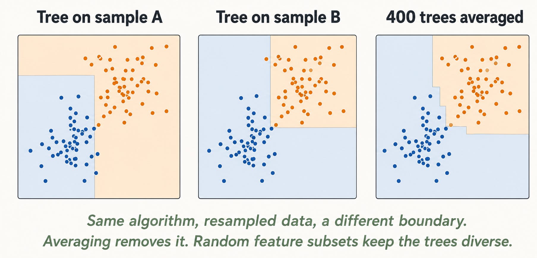
The problem is instability. Resample your data slightly and the top split can change, which changes every split below it. Two trees fit on 95% overlapping data can look nothing alike. Exploiting that turns out to be the whole game.

Two ways to combine trees

Ensembles of trees exist because a single tree fails in one of two ways, and there is a different fix for each.

A deep tree has low bias and high variance. It can carve the space finely enough to represent almost any function, so it is not systematically wrong about anything. But it is extremely sensitive to which rows it happened to see, so it is unreliable.
A shallow tree is the reverse: high bias, low variance. Stable across resamples, but too crude to capture the real shape.

That gives two strategies, and every model below is one of them.

Bagging attacks variance. Grow many deep trees on perturbed copies of the data, then average them. Individually unreliable, collectively stable.
Boosting attacks bias. Grow many shallow trees in sequence, where each one is fit to the errors the previous ones are still making, then add them all up. Individually useless, collectively sharp.

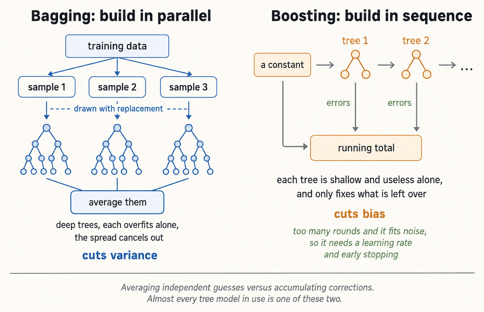
That is the entire taxonomy. What follows is variations on the details.

Bagging: grow deep trees in parallel and average them

The mechanism, concretely:

Draw a bootstrap sample: n rows sampled with replacement from your n rows. Some rows appear twice, and roughly 37% do not appear at all.
Grow a tree to full depth on that sample. No pruning. Let it overfit.
Repeat a few hundred times, independently.
To predict, average the predicted probabilities across all trees, or the means for regression.

Why averaging helps is worth being precise about, because it explains every design decision in this family. Average k independent estimators each with variance v and you get variance v/k, which goes to zero. But these trees are not independent, because they see mostly the same rows. If the typical pair of trees has correlation p, the variance of the average bottoms out at roughly p times v, no matter how many trees you add.

So the payoff comes from making the trees disagree, not from having more of them. Everything in this family is a trick for lowering p.

Averaging also leaves bias untouched, which is why the trees are deliberately grown deep. You want each one to be nearly unbiased and let the averaging clean up the noise.

Two practical consequences:

The trees are independent, so training parallelises across cores for free.
More trees never makes accuracy worse, it only costs time, so there is no overfitting knob to get wrong.

Random Forest

The default bagging implementation, and the model most likely to be good enough with no tuning at all.

How it works: bagging as above, plus one addition. At every single split, the tree is only allowed to consider a random subset of the features, max_features of them, conventionally the square root of the total for classification. It picks the best split among those, not among all.

from sklearn.ensemble import RandomForestClassifier

rf = RandomForestClassifier(
    n_estimators=500,
    max_features="sqrt",
    n_jobs=-1,
    random_state=42,
)
rf.fit(X_train, y_train)

Interesting feature: the feature subsampling is the real trick, not the bootstrap. Go back to the correlation p. If one feature dominates, every tree picks it at the root, every tree looks similar, p stays high, and averaging buys you very little. Restricting the candidates at each split forces different trees down different paths, which is what makes the average worth taking.

Three things worth knowing beyond that. Scikit-learn averages predicted probabilities rather than taking a majority vote, so the probabilities that come out are reasonably calibrated, which is unusual for an ensemble. Setting oob_score=True gives you a free validation estimate from the roughly 37% of rows each tree never saw, no holdout needed. And feature_importances_ is impurity based, which inflates high-cardinality features. Use permutation importance or SHAP when the ranking actually matters.

Extra Trees

A random forest with the split search deleted.

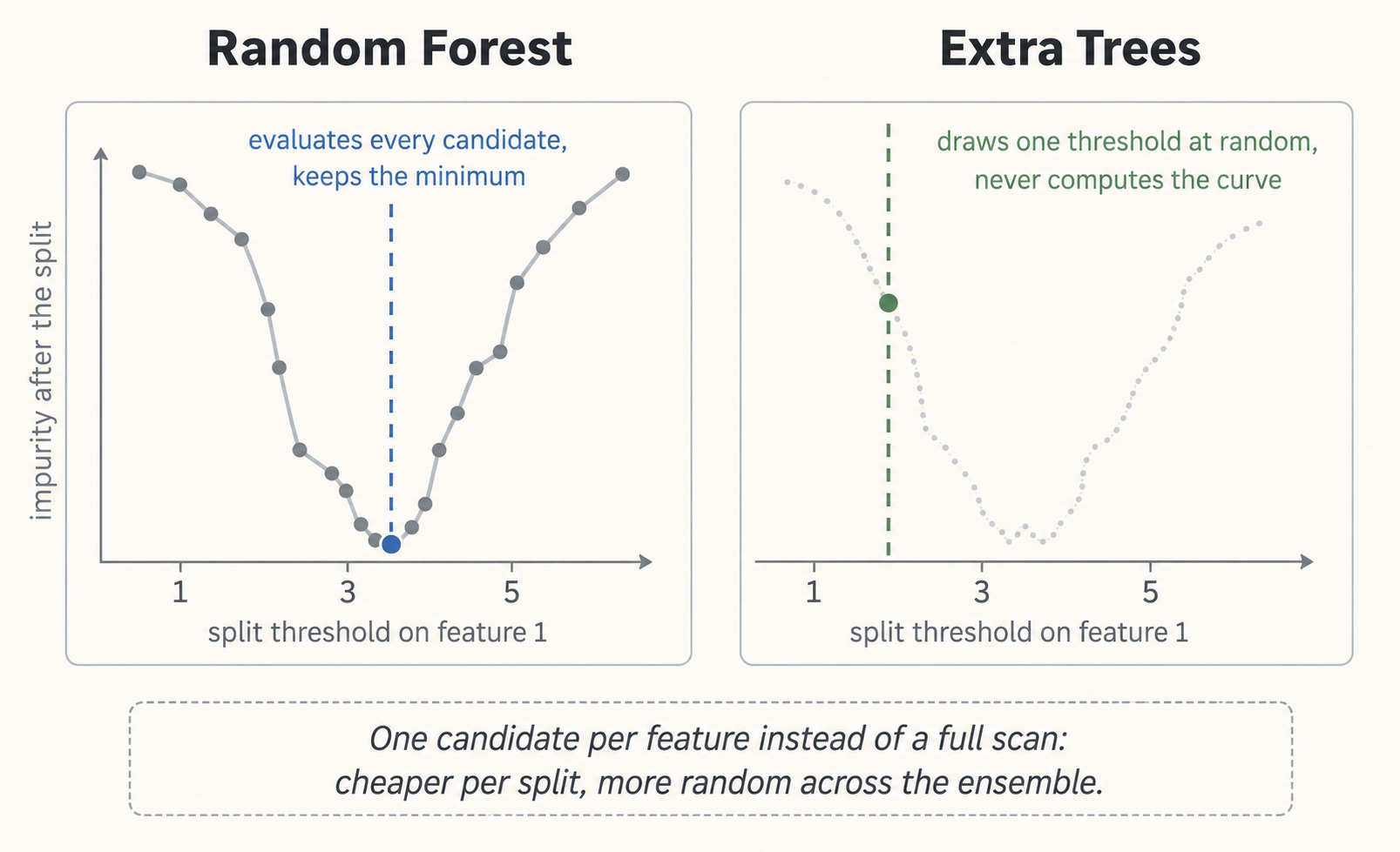
How it works: at each node, for each candidate feature, draw a single threshold uniformly at random from that feature’s range within the node. Score those few random splits and keep the best one. It never scans for an optimal cut point. By default it also skips the bootstrap and gives every tree the full dataset, since the random thresholds already supply the diversity.

from sklearn.ensemble import ExtraTreesClassifier

et = ExtraTreesClassifier(n_estimators=500, n_jobs=-1, random_state=42)
et.fit(X_train, y_train)

Interesting feature: skipping the search is both a speedup and a regulariser. Not searching means each split is a little worse, which raises bias slightly. But it also means the trees agree much less, which pushes that correlation p down and cuts variance further. On noisy data the trade is often favourable and it beats a forest outright. It costs nothing to fit both.

Boosting: grow shallow trees in sequence and add them up

Bagging builds trees that do not know about each other. Boosting builds each tree specifically to clean up after the ones before it.

The mechanism:

Start with a single constant prediction. The mean of y for regression, the log-odds of the base rate for classification.
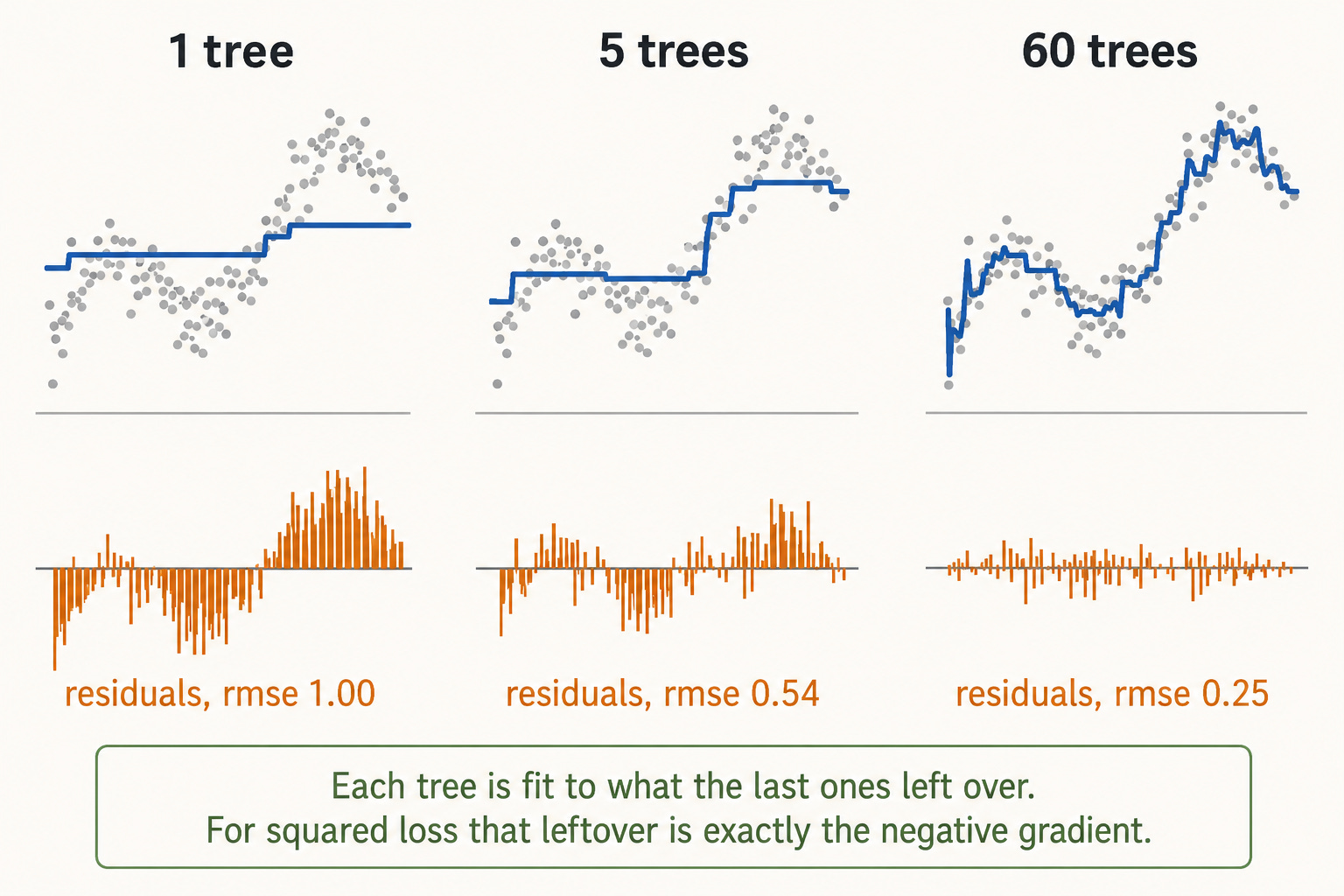
For every row, work out which direction the prediction needs to move to reduce the loss. For squared loss that is just y minus the current prediction, the residual. For log loss it is the label minus the predicted probability. In general it is the negative gradient of the loss with respect to the current prediction, which is where the name gradient boosting comes from.
Fit a small tree to that signal. Note what the tree is predicting: not y, but the correction.
Add a shrunk version of it to the running total. F = F + learning_rate * tree.
Go back to step 2 and repeat, now that the errors have changed.

So “fit the residuals” is exactly right for squared loss, and a good mental model for everything else. Formally each tree is one step of gradient descent, except the steps are taken in the space of functions rather than the space of parameters.

Why it reduces bias: each round targets the part of the signal the model cannot yet express, and chips away at it. Bagging averages away noise around a fixed level of expressiveness. Boosting keeps increasing the expressiveness.

Two consequences that matter every time you use one:

It is sequential. Tree 50 cannot start until tree 49 is done, so you cannot parallelise across trees, only inside a single split search. This is why the fast implementations obsess over the cost of one split.
It can overfit, and this is the real difference from bagging. Enough rounds and the model starts fitting noise. So the learning rate and the number of rounds trade off directly (halve the rate, roughly double the rounds) and you want a validation set with early stopping rather than a fixed round count.

AdaBoost

The original boosting algorithm, from 1995, and the clearest illustration of the idea. It predates the gradient framing entirely.

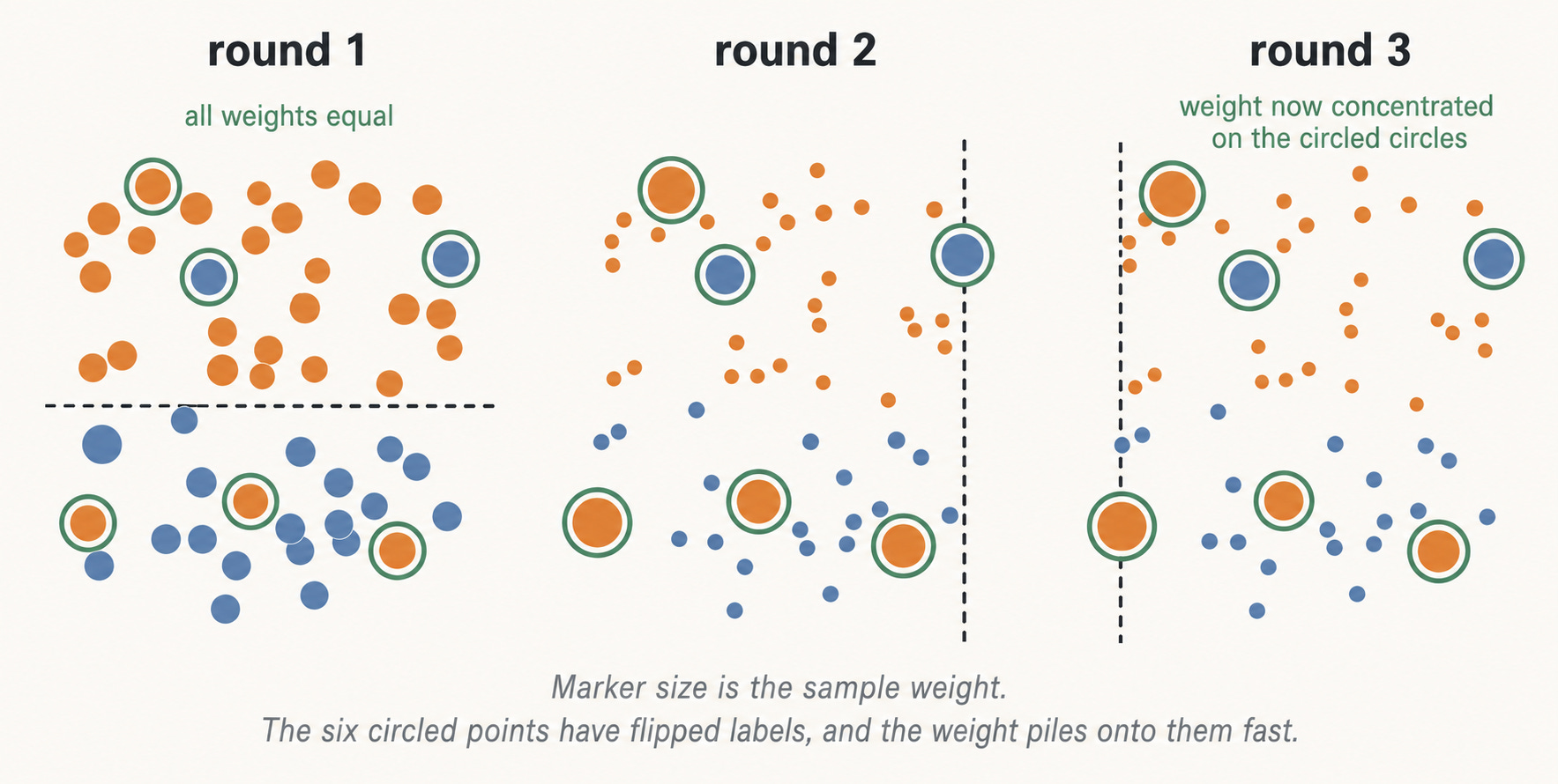
How it works: fit a stump on equally weighted rows. Find the rows it got wrong. Multiply their weights up and the correct ones down, renormalise, and fit the next stump on the reweighted data, which now cares mostly about the hard cases. Final prediction is a weighted vote, where the more accurate stumps get more say.

from sklearn.ensemble import AdaBoostClassifier

ada = AdaBoostClassifier(n_estimators=200, learning_rate=0.5)
ada.fit(X_train, y_train)

Interesting feature: reweighting and gradient fitting turn out to be the same algorithm. AdaBoost is gradient boosting with an exponential loss, which is a strong statement about its weakness. Exponential loss punishes confident mistakes brutally, so a mislabelled row gets upweighted round after round and the ensemble spends its capacity chasing it. That makes AdaBoost unusually sensitive to label noise, and it is why nobody reaches for it first any more.

Gradient Boosting

The general version. Swap the exponential loss for any differentiable loss and you get the algorithm from the section above, unmodified.

How it works: exactly steps 1 to 5, with an exact split search. At each node it sorts each feature and evaluates the gain at every possible cut point.

from sklearn.ensemble import GradientBoostingClassifier

gb = GradientBoostingClassifier(
    n_estimators=300,
    learning_rate=0.05,
    max_depth=3,
    subsample=0.8,
)
gb.fit(X_train, y_train)

Interesting feature: subsample below 1.0 fits each tree on a random fraction of rows, which is called stochastic gradient boosting. It regularises and speeds things up at the same time, and it is the one knob here worth setting away from its default.

The problem is scale. That exact split search costs time proportional to the number of distinct values in every feature, at every node, for every tree. Above roughly ten thousand rows this is the wrong implementation and you want the histogram version.

Histogram-based Gradient Boosting

The modern scikit-learn default, and the right first thing to try on tabular data. Heavily inspired by LightGBM.

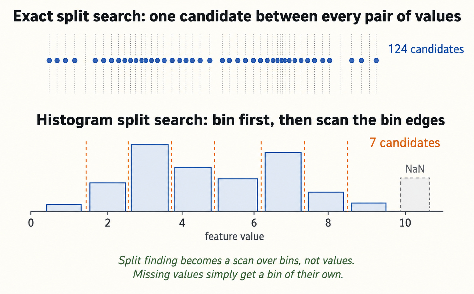
How it works: before any training, each continuous feature is bucketed once into a small number of bins, 255 for the observed values plus one reserved for missing. Every value is replaced by its bin index. Now a split search over a feature is a scan over bin boundaries instead of over distinct values, and the gradient sums per bin can be accumulated in a single pass over the rows. Cost per split stops depending on how many distinct values the feature has.

There is a second trick underneath: to get a child node’s histogram, compute the histogram of the smaller sibling and subtract it from the parent’s. One of the two children is always free.

from sklearn.ensemble import HistGradientBoostingClassifier

hgb = HistGradientBoostingClassifier(
    learning_rate=0.05,
    max_iter=500,
    max_leaf_nodes=31,
    categorical_features="from_dtype",
    early_stopping="auto",
)
hgb.fit(X_train, y_train)

Interesting feature: three things make this the sensible starting point.

Missing values are handled natively. NaNs get their own bin and the tree learns which side of each split to send them, so there is no imputation step and no leakage from imputing with training statistics.
Categorical features are handled natively too. Mark them with categorical_features, or use the pandas category dtype with "from_dtype", and it splits on subsets of categories directly with no one-hot expansion.
Early stopping is on by default once the dataset is large enough, so max_iter behaves like a ceiling rather than a number you have to tune.

It also supports monotonic constraints through monotonic_cst, which is how you force “raising the price never increases predicted conversion”. That is usually a hard requirement from the business rather than a nice-to-have.

XGBoost

The library that made boosted trees the default answer for tabular problems, and still the most tunable and most battle-tested of them.

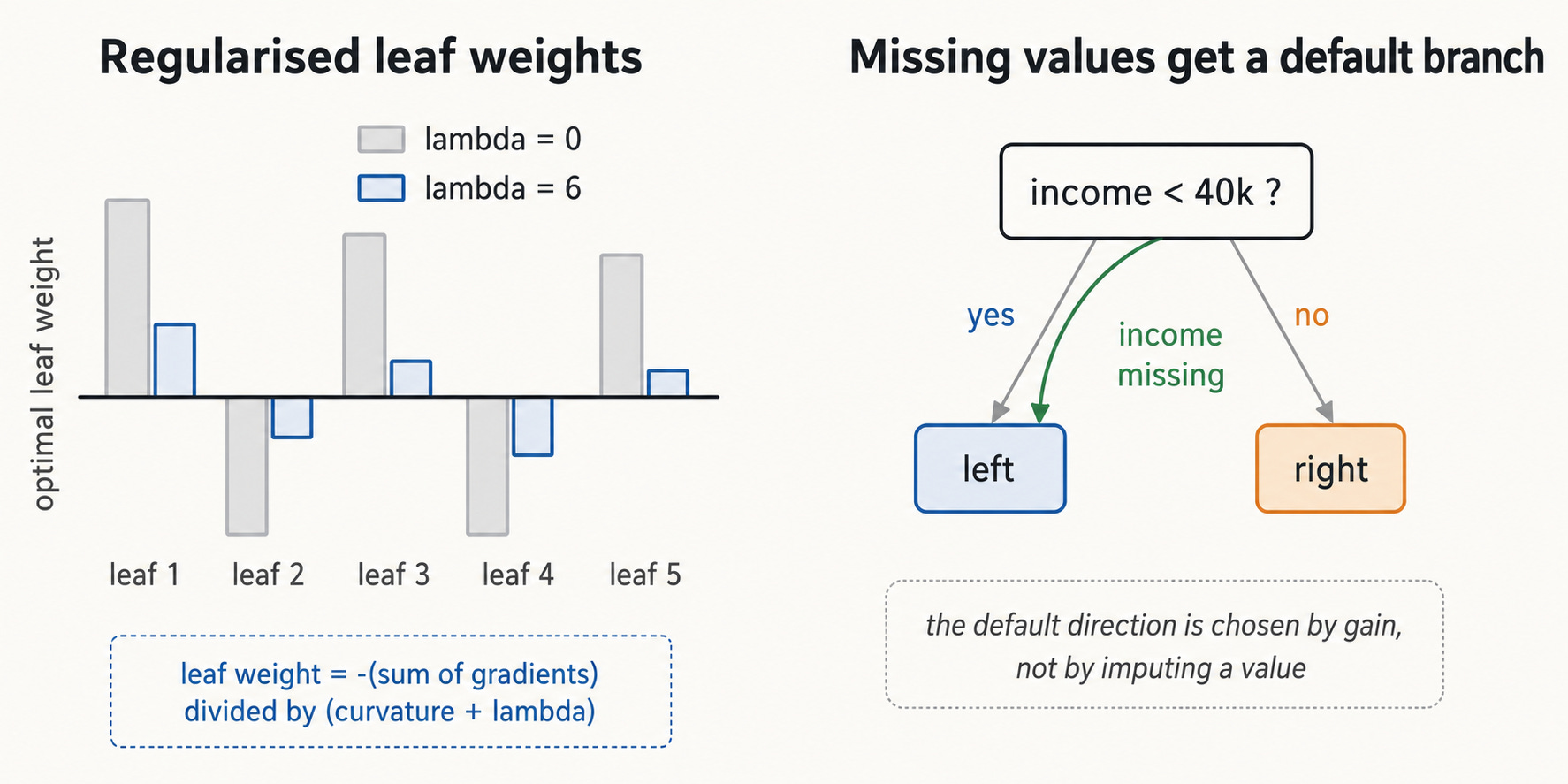
How it works: the same loop, but with a better local approximation. Instead of only using the gradient, XGBoost expands the loss to second order around the current prediction, so each node knows both the direction and the curvature. That quadratic has a closed-form solution, which gives an explicit formula for the best value to put in a leaf, and for the gain of any candidate split, with the regularisation term sitting in the denominator of both.

from xgboost import XGBClassifier

xgb = XGBClassifier(
    n_estimators=1000,
    learning_rate=0.05,
    max_depth=6,
    subsample=0.8,
    colsample_bytree=0.8,
    early_stopping_rounds=50,
    eval_metric="auc",
)
xgb.fit(X_train, y_train, eval_set=[(X_val, y_val)])

Interesting feature: because regularisation is inside the objective rather than applied afterwards, pruning is part of the optimisation. A split whose gain does not clear the penalty is simply never taken, and leaf values are shrunk toward zero automatically when a leaf holds little information.

Its other distinctive trick is sparsity-aware split finding. Missing and zero entries are skipped during the scan, and each node stores a learned default direction for them, chosen by gain. On sparse matrices this is a large speedup as well as a sensible way to handle absence.

LightGBM

The speed-focused option. Reach for it when the dataset is large and training time is the bottleneck.

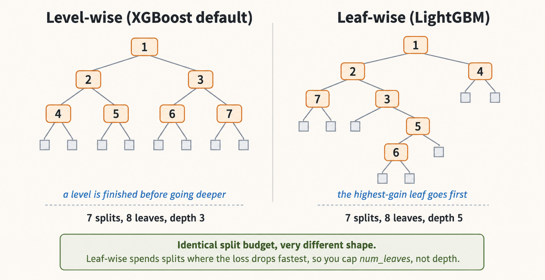
How it works: same second-order boosting, different growth strategy. Instead of finishing a whole level of the tree before going deeper, LightGBM keeps a queue of leaves and always splits whichever one promises the largest loss reduction, wherever it happens to sit. Trees come out deep and lopsided rather than balanced.

from lightgbm import LGBMClassifier

lgbm = LGBMClassifier(
    n_estimators=1000,
    learning_rate=0.05,
    num_leaves=63,
    colsample_bytree=0.8,
)
lgbm.fit(X_train, y_train, eval_set=[(X_val, y_val)])

Interesting feature: leaf-wise growth spends every split where it does the most good, so it reaches a given accuracy in fewer splits. The cost is overfitting risk, since nothing stops it driving one branch very deep on a handful of rows. That is why you tune num_leaves and min_child_samples here rather than max_depth, which is close to meaningless for an unbalanced tree.

It ships two more ideas aimed at speed. Gradient-based one-side sampling keeps all the rows with large gradients, the ones still being got wrong, and subsamples the rest. Exclusive feature bundling merges sparse features that are never nonzero together into a single feature, shrinking the effective width of the problem.

CatBoost

The one to reach for when your features are mostly high-cardinality categoricals: user IDs, postcodes, device models, merchant names.

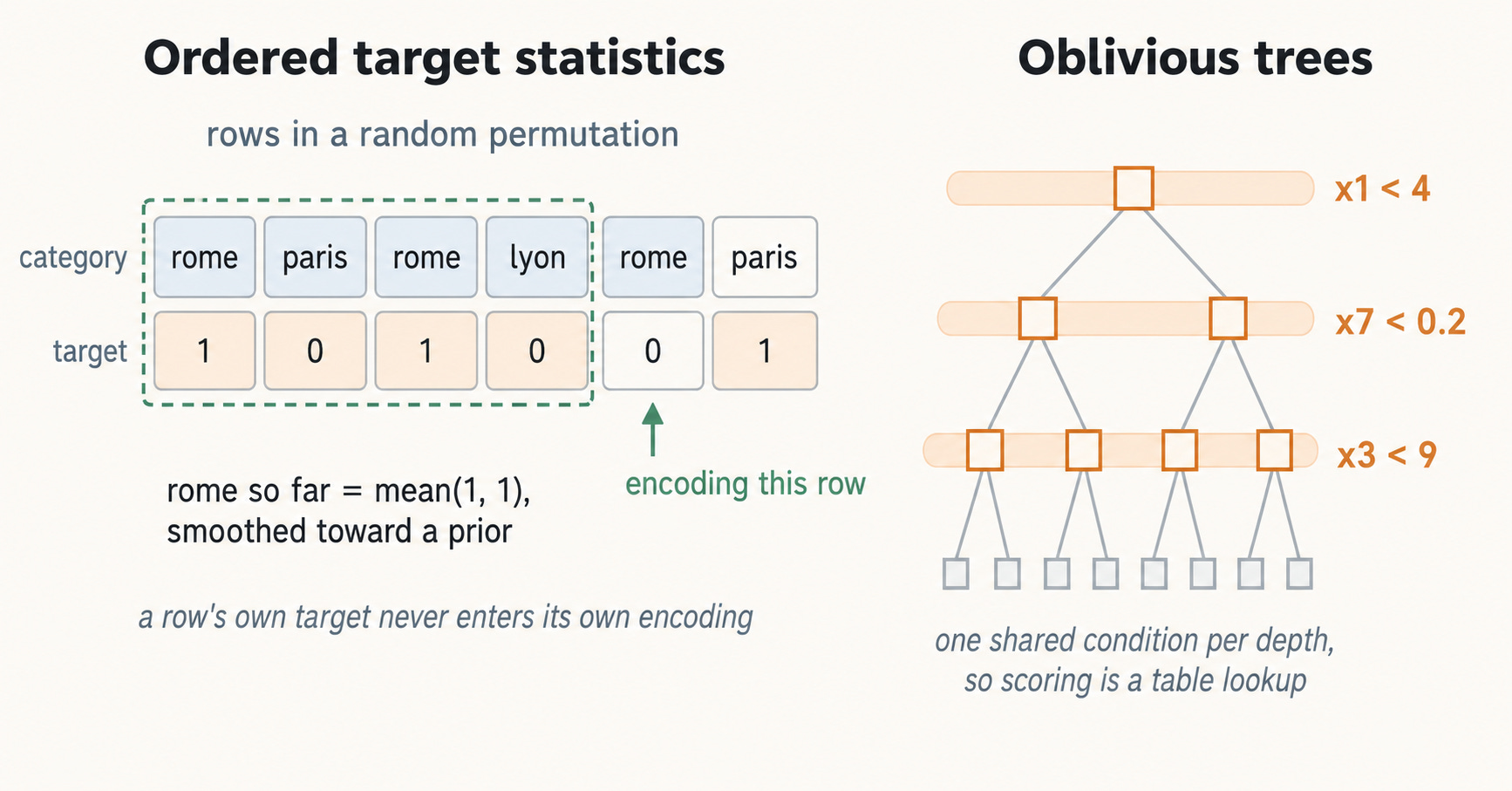
How it works: the usual boosting loop, with the category handling done carefully. Encoding a category by the mean target of its rows is the obvious move, and it leaks, because a row’s own label sits inside its own feature.

CatBoost fixes this by fixing a random permutation of the rows and computing each row’s encoding from earlier rows only, smoothed toward a global prior so a rare category is not encoded from a single observation.

It then applies the same logic to boosting itself, an approach called ordered boosting, to avoid the subtler leak where the residual you fit is computed by a model that has already seen the row.

from catboost import CatBoostClassifier

cb = CatBoostClassifier(
    iterations=1000,
    learning_rate=0.05,
    depth=6,
    cat_features=cat_cols,
    verbose=100,
)
cb.fit(X_train, y_train, eval_set=(X_val, y_val))

Interesting feature: its trees are oblivious, meaning every node at the same depth tests the same condition. That sounds like a pointless restriction, and it is a strong regulariser, but the real payoff is at serving time. A depth-6 oblivious tree is six comparisons producing a 6-bit index into a flat array of 64 leaf values, with no branching. If you are scoring millions of rows behind a latency budget, this matters more than a third decimal place of AUC.

Trees for other jobs

Not every tree ensemble predicts a label. Two worth knowing, because they reuse the same machinery for a different question.

Picking one

Start with HistGradientBoostingClassifier. It is fast, handles missing values and categoricals natively, needs no external dependency, and lands within a point or two of anything else on most datasets.

Discussion about this post

Ready for more?