Issue #139 - Bayesian Models: How Sure Are You?

💊 Pill of the Week

Your model says the conversion rate is 30%. Your stakeholder asks two things next: How sure are you, and what should we do about it?

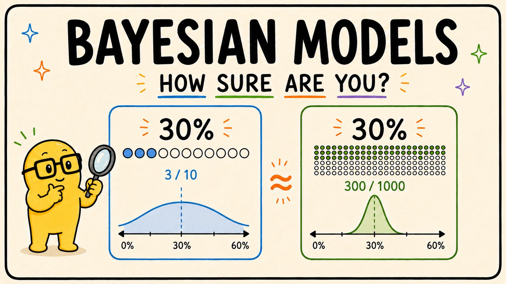
A single number answers neither. A Bayesian model answers both. That is the whole pitch. Everything else is plumbing.

The main idea

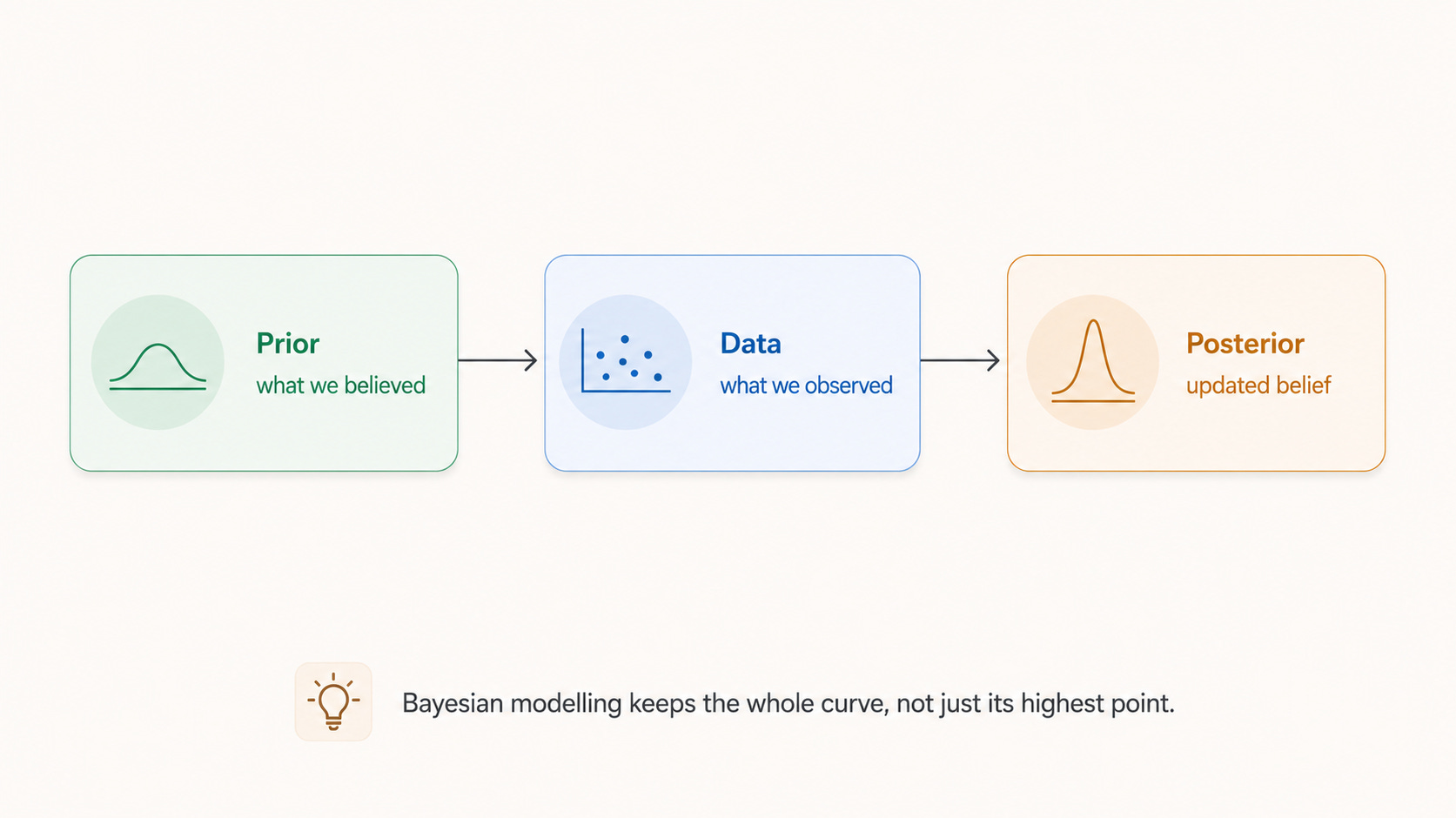
You start with a belief about some unknown quantity. You see data. You update the belief.

• The starting belief is called the prior.

• The data tells you how well each possible value explains what you saw, and that is the likelihood.

• The updated belief is the posterior.

The key difference from what you normally do is that the posterior is not a number. It is a whole curve over every possible value, with height meaning “how plausible is this?”. Regular ML hands you the single highest point of that curve and throws the rest away. Bayesian modelling keeps the curve.

The rest of this article is about why the curve is worth keeping.

---

Same number, very different confidence

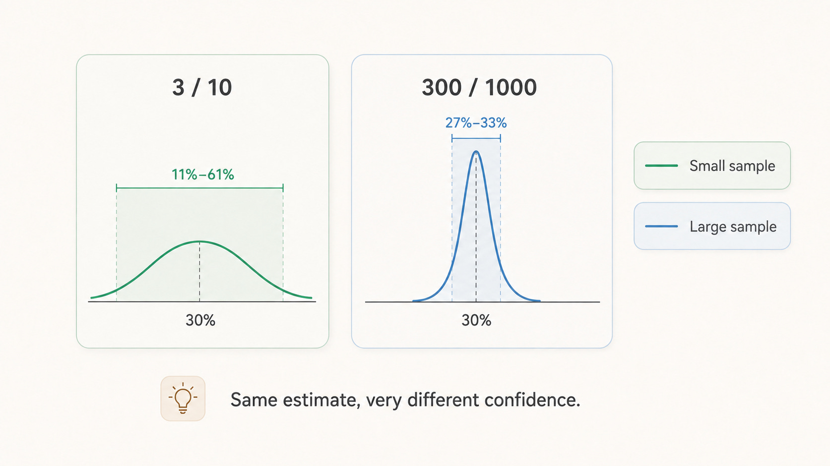
Two experiments both report a 30% conversion rate.

1. Run one: 3 conversions out of 10 visitors. The most likely value is 33%, but the range of values still plausible runs from 11% to 61%. That is basically the entire spectrum from “bad” to “amazing”.

2. Run two: 300 conversions out of 1000 visitors. The most likely value is 30%, with a plausible range of 27% to 33%. That range is nine times narrower.

Both go on the dashboard as 30%. One of them is a coin flip. Someone downstream is going to spend real money on that number.

Getting these ranges is not hard. For conversion-style data, the maths is a one-liner:

from scipy import stats

posterior = stats.beta(1 + conversions, 1 + visitors - conversions)

print(posterior.mean())                  # best guess
print(posterior.ppf([0.025, 0.975]))     # plausible range

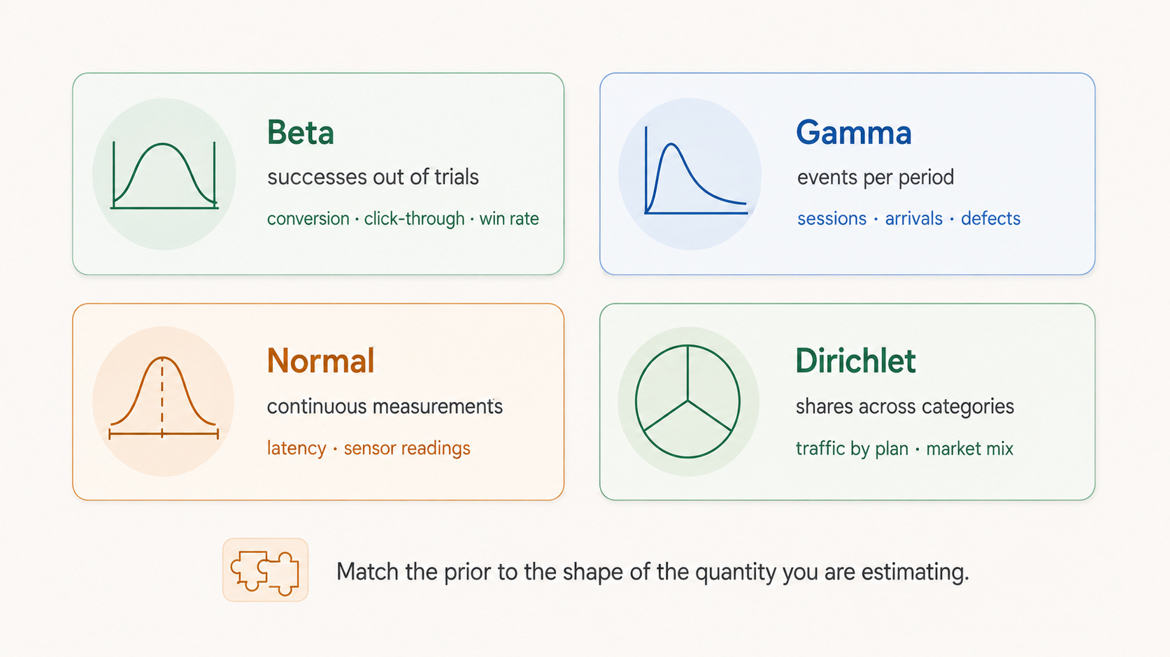
That is it. No sampling, no fitting loop. Certain combinations of prior and data have a closed-form answer, and this is one of them. They are called conjugate pairs, and there are four you will actually use:

• Counting successes out of trials, such as conversion, click-through and win rate: use a Beta prior.

• Counting events per period, such as sessions per user, arrivals and defects: use a Gamma prior.

• Averaging a continuous measurement, such as latency or sensor readings: use a Normal prior.

• Splitting a total into categories, such as share of traffic per plan: use a Dirichlet prior.

These distributions are not arbitrary. Each one matches the shape of the parameter being estimated and, when paired with the corresponding likelihood, gives a posterior of the same form. That is what makes the update cheap enough to do with simple arithmetic instead of a sampler.

These four cover a surprising amount of real work with no heavy machinery at all.

Why this range is the one people think they are getting

If you say “95% credible interval of 27% to 33%”, it means exactly what it sounds like: given the model, there is a 95% chance the true rate is in there.

A confidence interval, the frequentist version, does not mean that. It is a statement about how the procedure behaves if you repeated the experiment forever, not about your number. Almost nobody reads it that way.

So one practical benefit of going Bayesian is that you get to say the intuitive sentence and actually be right.

Turning the curve into a decision

Consider a paywall test using real numbers from a run I did for this article. Variant A had 71 conversions in 1200 impressions, so 5.92%. Variant B had 84 conversions in 1150 impressions, so 7.30%.

B looks better. But is it actually better, or did it get lucky? Draw a lot of samples from each posterior and just count:

from scipy import stats
import numpy as np

post_a = stats.beta(1 + 71, 1 + 1200 - 71)
post_b = stats.beta(1 + 84, 1 + 1150 - 84)

s_a, s_b = post_a.rvs(200_000), post_b.rvs(200_000)

print(np.mean(s_b > s_a))                     # 0.912
print(np.mean((s_b - s_a) / s_a > 0.10))      # 0.769
print(np.mean(np.maximum(s_a - s_b, 0)))      # 0.000416
print(np.mean(np.maximum(s_b - s_a, 0)))      # 0.014286

That gives you four useful statements you can put straight into a Slack message:

• There is a 91% chance B is better than A.

• There is a 77% chance B is better by at least 10%.

• The best guess for the improvement is 23%, though it could plausibly be anywhere from slightly negative to 59%.

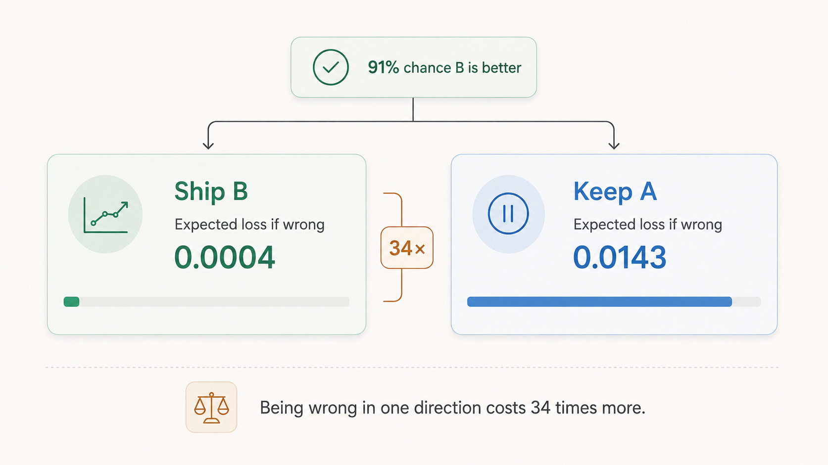
• If we ship B and we are wrong, we lose about 0.0004 conversions per impression. If we keep A and we are wrong, we lose 0.0143.

The last comparison is the important one. Being wrong in one direction is 34 times more expensive than being wrong in the other.

That is what ends the meeting.

This idea is called expected loss, and it is simply “how much do I lose on average if this choice turns out to be the bad one?”. You ship when the expected loss of shipping drops below a threshold you picked from actual business cost.

Worth noting: this test never hit p < 0.05. The Bayesian read still says ship.

There is a second perk. You can look at the results whenever you want. Today’s posterior becomes tomorrow’s prior, so checking early does not break anything. In classical testing, peeking inflates your false positive rate and you need extra corrections to stay honest.

Priors, and why they are less scary than they sound

The usual objection is that priors let you put your thumb on the scale. But you are already doing it. L2 regularisation is exactly a prior saying “weights are probably near zero”. L1 is a different prior with the same job. Early stopping is a prior you never wrote down. Bayesian modelling simply makes the assumption visible so someone can argue with it.

Four rules keep you out of trouble:

1. Do not use a flat prior by default. “Anything is equally possible” sounds neutral, but it is not. It puts real weight on conversion rates of 99%. Something mildly opinionated like “probably between 1% and 20%” is both more honest and better behaved.

2. Simulate before you fit. Draw parameters from your prior, generate fake data and look at it. If the fake data is absurd, your prior is absurd. This takes five minutes and catches most mistakes.

3. Write the prior in units you understand. “Typical conversion is somewhere around 5%” is easy to sanity check. The same thing expressed in log odds is not.

4. Try a tighter one and a looser one. If your conclusion flips, the data is not doing the work. Better to find that out now than in the review.

One reassuring fact is that with a decent amount of data, the prior barely matters because the data overwhelms it. The prior only really moves things when you have very little data, which is exactly when you wanted help.

The technique that earns its keep: borrowing strength

This is the part I would actually put in production first.

You have eight paywall variants. Four have thousands of impressions, while four have barely any. The small ones show wild rates that are mostly noise, and whichever one got lucky ends up at the top of your ranking.

Your two obvious options are both bad. Lump everything together and you erase real differences. Score each variant on its own and you are trusting 14 conversions out of 95 visitors.

A hierarchical model does neither. Every variant gets its own rate, but all the rates are assumed to come from a shared pool. In practice, that means a variant with little data gets pulled towards what the other variants are doing, while a variant with lots of data is left largely alone. Small groups borrow strength from the group as a whole.

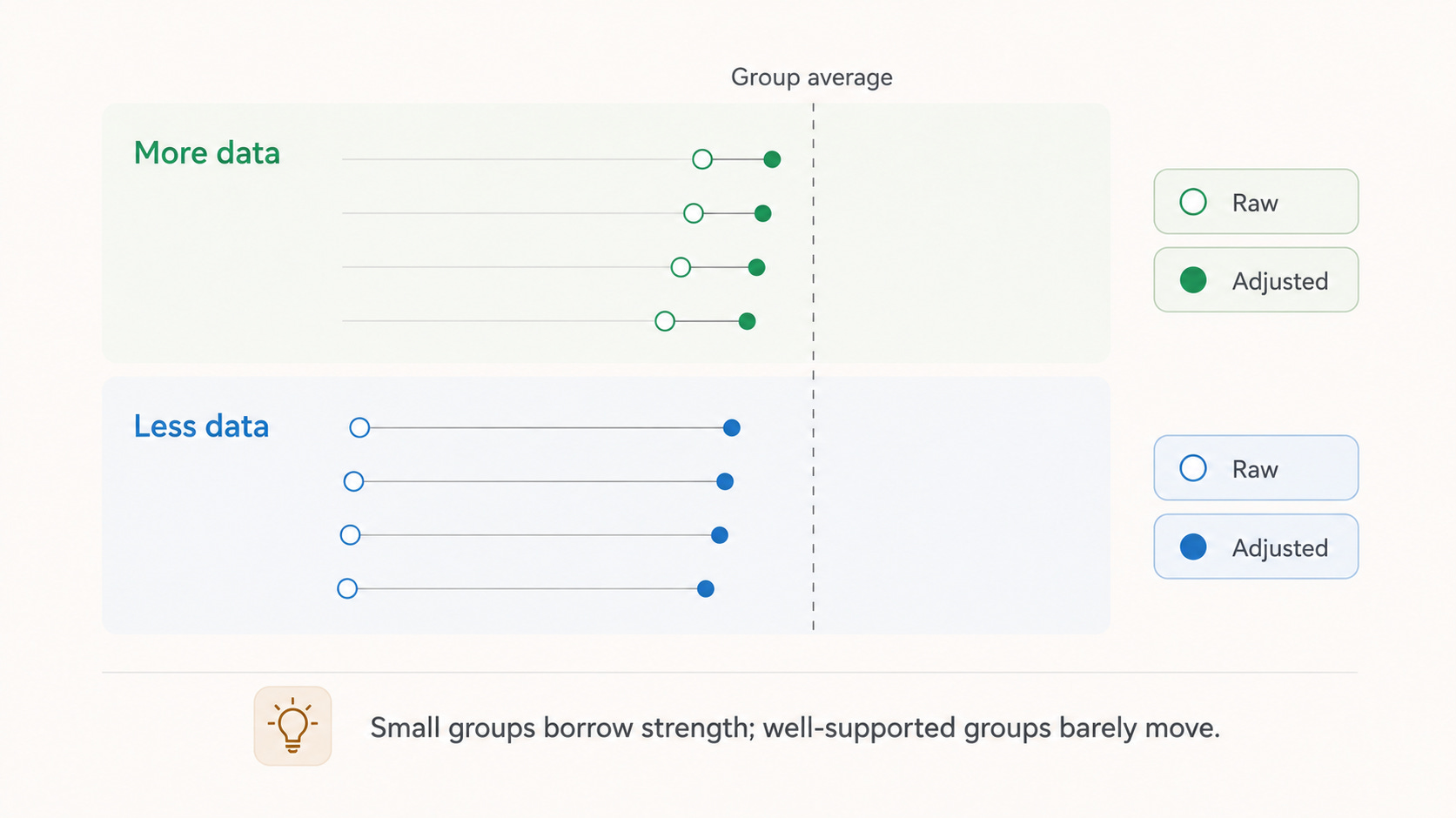
For the four large variants, almost nothing changes:

• annual_v1: 4,200 impressions, raw 5.50%, adjusted 5.57%.

• annual_v2: 3,900 impressions, raw 6.90%, adjusted 6.91%.

• monthly_v1: 5,100 impressions, raw 5.90%, adjusted 5.95%.

• monthly_v2: 4,800 impressions, raw 5.10%, adjusted 5.18%.

With thousands of impressions, each variant is its own best evidence.

Now look at the four small variants:

• trial_7d: 900 impressions, raw 8.00%, adjusted 7.92%, plausible range 6.3% to 9.7%.

• trial_14d: 260 impressions, raw 10.00%, adjusted 9.18%, plausible range 6.4% to 12.7%.

• bundle: 180 impressions, raw 10.00%, adjusted 9.00%, plausible range 6.0% to 13.0%.

• winback: 95 impressions, raw 14.74%, adjusted 10.86%, plausible range 6.5% to 17.4%.

winback is the story. On raw numbers it is your best paywall by a mile, and someone is about to reallocate budget to it. After adjustment it drops to 10.9%, while its plausible range still stretches from 6.5% to 17.4%. That is an honest description of what 14 conversions can tell you.

The pull towards the group average is called shrinkage, and the nice part is that you do not choose how much of it to apply. The model works it out from how different the groups genuinely are. Groups that really do behave differently get left alone. Groups that look different only because of small samples get pulled in.

Anywhere you have many small groups, this applies: users, stores, regions, cohorts, SKUs, test arms and sensors.

When you need a real sampler

Once you add covariates or several layers, the closed-form solutions stop working. Then you sample the posterior instead of computing it. The tooling for this is much friendlier than its reputation:

import pymc as pm

with pm.Model() as model:
    # the shared pool
    mu    = pm.Beta("mu", 2, 20)          # typical conversion rate across variants
    kappa = pm.HalfNormal("kappa", 200)   # how tightly variants cluster around it

    # one rate per variant
    theta = pm.Beta("theta", mu * kappa, (1 - mu) * kappa, shape=n_variants)

    pm.Binomial("obs", n=n_obs, p=theta, observed=k_obs)

    idata = pm.sample(
        2000,
        tune=2000,
        target_accept=0.9,
        chains=4,
        random_seed=42
    )

That is roughly ten lines for a full hierarchical model. In terms of libraries:

• PyMC is the friendliest and where I would start.

• NumPyro is the fast one, built on JAX. Use it when PyMC gets slow.

• Stan is the reference implementation with excellent diagnostics, but it is a separate language to learn.

• Variational inference (pm.fit in PyMC) is the fast approximation. It is fine for iterating, but it tends to report intervals that are too narrow, so be careful if the interval was the point.

If sampling is too slow for your use case, there are cheaper approximations. A bootstrap over an ensemble gives you rough uncertainty for almost nothing. It is less principled, but often good enough.

Paid subscribers get the practical part:

• the four checks that reveal whether a Bayesian model can be trusted

• plus how to turn uncertainty into better exploration

• stopping rules and money-based decisions.

• You’ll also get the reproducible Python code behind every result.