Issue #91 - Principal Component Analysis (PCA)

💊 Pill of the Week

Principal Component Analysis (PCA) is a fundamental dimensionality reduction technique widely used in data science, machine learning, and statistics. It transforms high-dimensional data into a lower-dimensional space while preserving as much information as possible. In this article, we'll explore how PCA works, its applications, advantages, limitations, and how to implement it in Python.

💎For the paid subscribers also how to choose the number of components!

How Does PCA Work?

PCA is essentially a mathematical procedure that transforms a set of correlated variables into a set of uncorrelated variables called principal components. These principal components are ordered so that the first few retain most of the variation present in all of the original variables.

Step-by-Step Process:

1. Standardization: First, the data is standardized to have a mean of 0 and a standard deviation of 1. This step is crucial because PCA is sensitive to the scale of the variables.

2. Covariance Matrix Computation: The covariance matrix is calculated to understand how variables change together.

3. Eigenvalue Decomposition: The covariance matrix is decomposed into eigenvectors and eigenvalues.

   • Eigenvectors determine the direction of the new feature space.

   • Eigenvalues determine the magnitude of variability in the direction of the eigenvectors.

4. Principal Components Selection: Eigenvectors are sorted by eigenvalues in descending order, and the top k eigenvectors are chosen to form a matrix of principal components.

5. Transformation: Finally, the original dataset is transformed into the new k-dimensional space.

Key Concepts:

Principal Components

Principal components are new variables that are created as linear combinations of the original variables. They are uncorrelated with each other and ordered by the amount of variance they explain.

Variance Explained

Each principal component explains a certain percentage of the total variance in the data. The first principal component explains the most variance, the second explains the second most, and so on.

Dimensionality Reduction

By keeping only the first few principal components (those that explain most of the variance), we can reduce the dimensionality of our data while retaining most of the information.

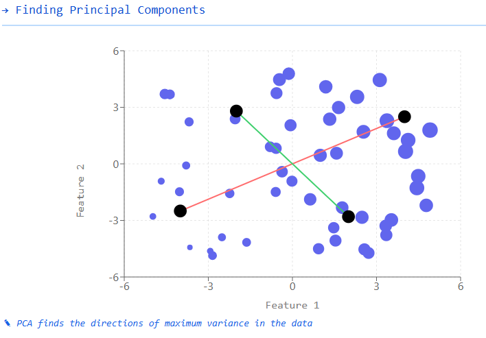
Visual Explanation of PCA

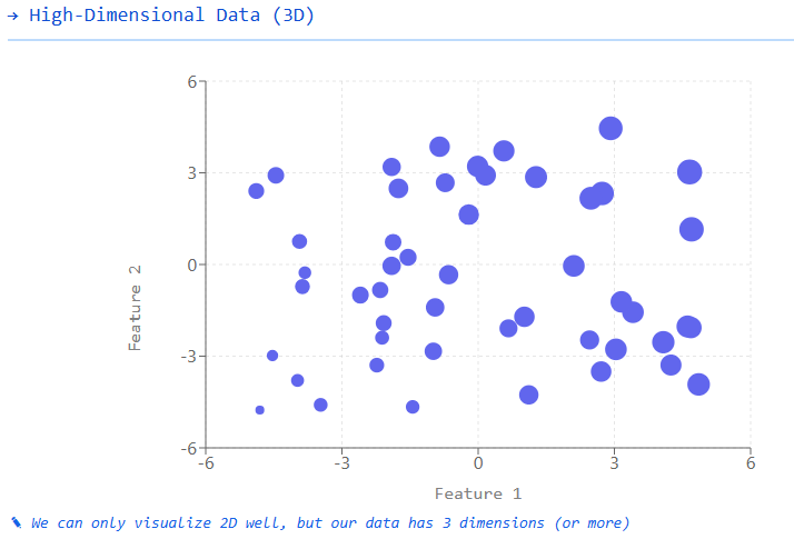
Consider a 3D dataset where each point represents a sample with three features:

1. Original Data: Points are scattered in a 3D space with three axes (features).

   

2. Find Principal Components:

   • The first principal component (PC1) is the direction of maximum variance in the data.

   • The second principal component (PC2) is perpendicular to PC1 and captures the next highest variance.

     

     

3. Project Data: The original 3D data is projected onto the new coordinate system defined by PC1, PC2, and PC3.

   

4. Dimensionality Reduction:

   • If we keep only PC1 and PC2, we reduce our data from 3D to 2D, preserving most of the variance.

   • If we keep only PC1, we further reduce the data from 3D to 1D, while retaining the highest variance component.

When to Use PCA?

PCA is particularly useful in the following scenarios:

1. High-Dimensional Data: When dealing with datasets with many features that might lead to overfitting.

2. Visualization: To visualize high-dimensional data in 2D or 3D.

3. Noise Reduction: To filter out noise in the data by focusing on components with higher variance.

4. Feature Extraction: To extract meaningful features from complex data.

5. Multicollinearity: When dealing with highly correlated features in regression models.

Pros and Cons

Pros:

• Dimensionality Reduction: Reduces computational complexity and memory usage.

• Removes Multicollinearity: Creates uncorrelated features.

• Noise Reduction: Can help filter out noise in the data.

• Visualization: Makes high-dimensional data visualizable.

Cons:

• Interpretability: Principal components can be difficult to interpret as they are combinations of original features.

• Linear Assumptions: Only captures linear relationships between features.

• Data Scaling Sensitivity: Results are sensitive to the scale of the input features.

• Information Loss: Some information is inevitably lost when reducing dimensions.

Python Implementation

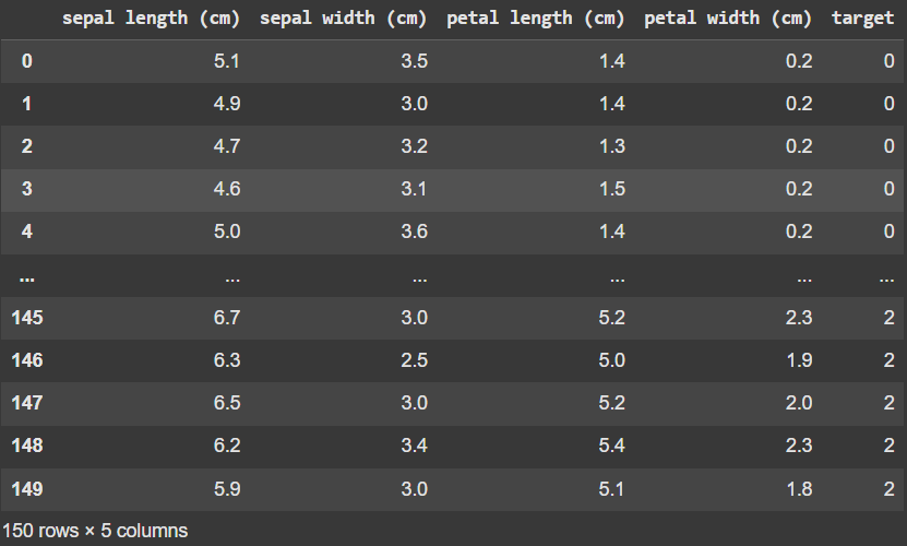
Let's implement PCA using scikit-learn. We will use the iris dataset (💎how to load it at the end of the issue):

from sklearn.decomposition import PCA
from sklearn.preprocessing import StandardScaler
import numpy as np
import matplotlib.pyplot as plt

# Standardize the data and apply PCA
pca = PCA(n_components=2)

# Reduce to 2 dimensions
X_pca = pca.fit_transform(X_scaled)

To interpret the results we can visualize the resulting values (💎code at the end of the issue).

Also we can get the explained variance by the selected components:

# Explained variance
print(f"Explained variance ratio: {pca.explained_variance_ratio_}")
print(f"Total explained variance: {sum(pca.explained_variance_ratio_):.2f}")

Explained variance ratio: [0.72962445 0.22850762]
Total explained variance: 0.96

We applied PCA to the Iris dataset using scikit-learn. Here’s what we get:

1. Dimensionality Reduction

• The original dataset has 4 features (sepal length, sepal width, petal length, petal width).

• PCA reduces it to 2 principal components while retaining 96% of the variance.

2. Standardization

• The data is standardized using StandardScaler() to ensure that all features have a mean of 0 and unit variance.

• Standardization is crucial for PCA because PCA is sensitive to different feature scales.

3. Principal Components and Visualization

• The dataset is transformed into a new coordinate system based on the two principal components.

• The scatter plot shows the Iris dataset in the 2D PCA space, where:

  • Red (r): Setosa

  • Green (g): Versicolor

  • Blue (b): Virginica

• The separation between classes indicates that PCA captures most of the structure in the data.

4. Explained Variance

• pca.explained_variance_ratio_ tells us how much variance each principal component captures:

  • PC1: 72.96%

  • PC2: 22.85%

• The total explained variance is 96%, meaning we retain most of the dataset's original information in just two dimensions.

Interpreting the Results

Key outputs from a PCA model include:

1. Transformed Data: The original data projected onto the principal components.

2. Components: The principal components themselves, which are the eigenvectors of the covariance matrix.

3. Explained Variance Ratio: The proportion of variance explained by each principal component.

4. Singular Values: Related to the square roots of the eigenvalues of the covariance matrix.

Here's how you can extract these outputs:

# Extract components 
components = pca.components_ 
print("Principal Components:") 
print(components) 

# Explained variance ratio for each component 
explained_variance = pca.explained_variance_ratio_ 
print("\nExplained Variance Ratio:") 
print(explained_variance) 

# Create a scree plot to visualize explained variance 
plt.figure(figsize=(10, 6)) 
plt.bar(range(1, len(explained_variance) + 1), explained_variance, alpha=0.5, align='center') 
plt.step(range(1, len(explained_variance) + 1), np.cumsum(explained_variance), where='mid') 
plt.ylabel('Explained variance ratio') 
plt.xlabel('Principal Components') 
plt.title('Scree Plot') 
plt.show()

Principal Components:
[[ 0.52106591 -0.26934744  0.5804131   0.56485654]
 [ 0.37741762  0.92329566  0.02449161  0.06694199]]

Explained Variance Ratio:
[0.72962445 0.22850762]

1. Principal Components

• These are the eigenvectors of the covariance matrix, which define the new feature space.

• The printed principal components matrix shows how the original features contribute to each principal component:

  \( \begin{bmatrix} 0.521 & -0.269 & 0.580 & 0.565 \\ 0.377 & 0.923 & 0.024 & 0.067 \end{bmatrix} \)

  Interpretation:

  • The first principal component (PC1) has strong positive weights for petal length and petal width.

  • The second principal component (PC2) is dominated by sepal width.

2. Explained Variance Ratio

• Indicates how much of the total variance is captured by each principal component:

  \( [0.7296, 0.2285]\)

  Interpretation:

  • PC1 captures 72.96% of the total variance.

  • PC2 captures 22.85% of the total variance.

  • Together, the two components retain 96% of the dataset’s original structure.

3. Scree Plot

• The scree plot visualizes the explained variance ratio.

• The bar chart shows the variance captured by each component.

• The step line represents the cumulative variance across components.

• From the plot, we can see that two components are enough to capture most of the variance. It shows that PC1 explains ~73% and PC2 ~23% of the variance, totaling ~96%. The cumulative variance curve confirms that two components capture almost all the information, justifying dimensionality reduction to 2D.

Real-World Applications

1. Image Compression: Reducing the dimensions of image data while preserving important features.

2. Facial Recognition: Extracting key features from facial images (Eigenfaces).

3. Genome Data Analysis: Analyzing gene expression data and identifying patterns.

4. Finance: Risk management and portfolio optimization.

5. Anomaly Detection: Identifying outliers in high-dimensional data.

6. Natural Language Processing: Semantic analysis and document classification.

7. Data Visualization: Reducing high-dimensional data to 2D or 3D for better interpretability.

Common Variants of PCA

1. Kernel PCA: This variant extends PCA by using kernel methods, enabling it to capture nonlinear relationships in data. By applying a kernel trick (like the Radial Basis Function kernel), Kernel PCA transforms the data into a higher-dimensional space where linear separation may be more effective. It’s particularly useful when data is not linearly separable in its original form.

2. Incremental PCA: For large datasets that don’t fit into memory, Incremental PCA computes principal components in a batch-wise manner, processing data in smaller chunks. This makes it more memory-efficient while still benefiting from PCA’s dimensionality reduction capabilities.

3. Sparse PCA: Sparse PCA introduces sparsity into the principal components, encouraging many of the coefficients in the components to be zero. This leads to simpler, more interpretable components, which can be especially helpful when the goal is to identify key features or understand the structure of the data.

4. Robust PCA: Robust PCA is designed to be less sensitive to outliers in the data. It typically uses a robust loss function to reduce the influence of outliers, making it suitable for real-world datasets where noise or extreme values might distort the results of standard PCA.

Each variant of PCA is designed to address different challenges, offering more flexibility and robustness depending on the nature of the data you're working with.

Conclusion

Principal Component Analysis is a powerful technique for dimensionality reduction and feature extraction. By transforming high-dimensional data into a lower-dimensional space, PCA helps to simplify complex datasets while retaining most of the important information. Although it has some limitations, PCA remains a fundamental tool in the data scientist's toolkit.

Understanding how PCA works and when to apply it can significantly enhance your data analysis capabilities, allowing you to extract meaningful insights from complex high-dimensional data and improve the performance of machine learning models.

---

‍🎓Further Learning*

Let us present: “From Beginner to Advanced LLM Developer”. This comprehensive course takes you from foundational skills to mastering scalable LLM products through hands-on projects, fine-tuning, RAG, and agent development. Whether you're building a standout portfolio, launching a startup idea, or enhancing enterprise solutions, this program equips you to lead the LLM revolution and thrive in a fast-growing, in-demand field.

Who Is This Course For?

This certification is for software developers, machine learning engineers, data scientists or computer science and AI students to rapidly convert to an LLM Developer role and start building

*Sponsored: by purchasing any of their courses you would also be supporting MLPills.

---

⚡Power-Up Corner

Choosing the Number of Components

One critical decision when using Principal Component Analysis (PCA) is determining how many principal components to retain. Selecting too few components may result in information loss, while keeping too many may lead to unnecessary complexity. Here are some common approaches:

• Explained Variance Threshold – Retain enough components to explain a predefined percentage (e.g., 95%) of the total variance.

• Kaiser Criterion – Keep components with eigenvalues greater than 1.

• Scree Plot – Identify the "elbow" point in the explained variance vs. number of components plot.

• Cross-Validation – Use model performance (e.g., classification accuracy) to select the optimal number of components.

• Parallel Analysis (Horn’s Method) – Compare actual eigenvalues with those from randomly generated data to determine significant components.

Let’s see them in detail:

1. Explained Variance Threshold

• A common heuristic is to retain enough principal components to explain a predefined percentage of the total variance, such as 90% or 95%. This ensures that the retained components capture most of the dataset’s information while reducing dimensionality.

# Determine number of components that explain 95% of variance 
pca_full = PCA().fit(X_scaled) 
cumsum = np.cumsum(pca_full.explained_variance_ratio_) 
d = np.argmax(cumsum >= 0.95) + 1 
print(f"Number of components needed to explain 95% of variance: {d}")

Number of components needed to explain 95% of variance: 2

2. Kaiser Criterion