Issue #92 – Decision Trees

💊 Pill of the Week

Decision Trees (DTs) are a non-parametric supervised learning method used for both classification and regression tasks. They model decisions in a flowchart-like tree structure, mimicking how humans make choices through a series of questions or tests. In a decision tree, each internal node represents a question or test on a feature (e.g., “Is age > 30?”), each branch represents an outcome of that test (e.g., yes/no), and each leaf node represents a final decision or prediction (a class label or numerical value).

This intuitive structure makes decision trees easy to understand and interpret – even for non-experts – which is a key reason they are among the most popular machine learning algorithms. Whether predicting if a patient has a disease or if a customer will churn, decision trees provide a transparent decision-making framework that clearly lays out why a prediction was made.

Why are decision trees important?

In addition to their interpretability, decision trees can handle diverse data types (both numerical and categorical features) and require relatively little data preprocessing. They partition data based on feature values, recursively splitting the dataset into homogenous subsets. This “divide and conquer” approach means that decision trees can capture complex nonlinear relationships in the data without assuming a particular functional form.

They also form the foundation of more advanced ensemble methods like Random Forests and Gradient Boosted Trees, which build upon decision tree learners to achieve state-of-the-art performance in many domains. In sum, decision trees are a fundamental and versatile tool in the machine learning toolkit, balancing simplicity and power in solving real-world problems.

Core Concepts

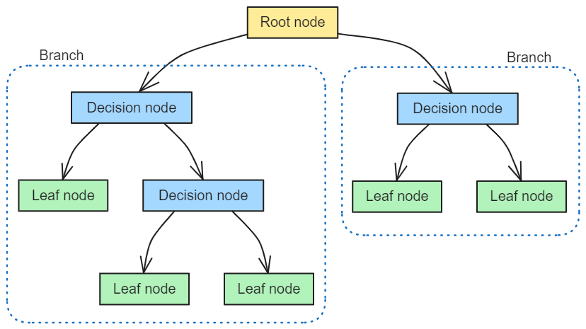
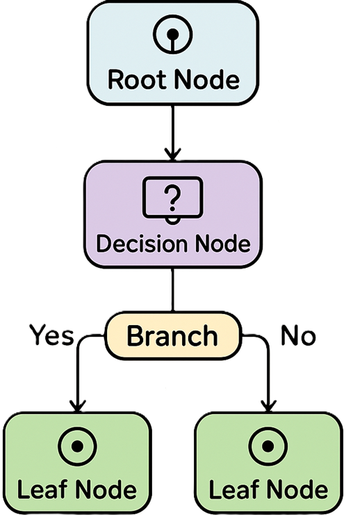
• Root Node: The top node of the tree, representing the entire dataset (population) before any splitting. This node will eventually split on the feature that best separates the data.

• Decision Node (Internal Node): A node that splits into two or more sub-nodes. Each decision node poses a question (condition) on a feature and branches out based on the answer.

• Branch: The connector between nodes, representing the outcome of a decision or test. For example, a branch might correspond to “Feature X > 5” being true vs false.

• Leaf Node (Terminal Node): A node that has no further splits​. Leaves output a prediction – e.g. a class label in classification, or a numeric value in regression. Each leaf can be seen as a final decision or outcome for instances that follow the path from the root to that leaf.

• Parent and Child Nodes: In the tree hierarchy, any node that splits into sub-nodes is the parent of those sub-nodes (its children)​. The root is the ultimate parent, and the leaves are children with no offspring of their own.

• Splitting: The process of dividing a node into two or more sub-nodes based on a feature’s value. The goal is to create purer subsets that are more homogeneous in terms of the target variable.

• Pruning: The process of removing sub-nodes (trimming the tree) to prevent over-complexity​. Pruning helps in simplifying the model and avoiding overfitting by cutting back sections of the tree that provide little predictive power.

---

📖 Book of the week

If you're working with time-based data — whether in finance, supply chain, energy, or tech — you need to check it out:

"Modern Time Series Forecasting with Python (2nd Edition)" By Manu Joseph & Jeffrey Tackes

This book isn’t just another walkthrough — it’s a complete toolkit that blends classic forecasting with the latest advancements in AI. Whether you’re tackling short-term demand spikes or long-term trends, it offers a solid path from fundamentals to production-ready solutions.

What sets it apart?

It bridges the gap between classical statistical methods and cutting-edge machine learning, so you're not choosing between the old and the new — you're mastering both:

• Learn foundational approaches like ARIMA, exponential smoothing, and seasonal decomposition

• Build advanced models using deep learning, transformers, and N-BEATS

• Explore probabilistic forecasting, global models, ensemble techniques, and conformal prediction

• All powered by hands-on Python code with PyTorch, pandas 2.0, and scikit-learn

This is a must-read for

• Data scientists

• Analysts

• ML engineers

• Researchers tackling time-driven problems

If you’re ready to take your forecasting skills beyond the basics — and want to explore what’s next in time series with deep learning and ML — this is the book for you.

---

How does a decision tree make decisions?

It all comes down to choosing the right splits. The tree is built top-down (starting from the root) by recursively splitting the data. At each decision node, the algorithm must decide which feature and what threshold (for numeric features) or category (for categorical features) to split on.

This choice is made by optimizing a splitting criterion – a quantitative measure of how well a given split separates the data into pure subsets. Two common impurity measures used in classification trees are:

• Entropy: a measure from information theory that quantifies the disorder or uncertainty in a dataset. Entropy is zero if all examples in a node are of the same class (pure), and higher when classes are mixed. Mathematically, for a node with class distribution p1, p2,...,pC, entropy is

  \(H(p) = -\sum_{i=1}^{C} p_i \log_2 p_i\)

• Gini Impurity: the probability of misclassifying a randomly chosen element from the node if we label it according to the node’s class distribution. It’s calculated as

  \(G(p) = \sum_{i=1}^{C} p_i (1 - p_i)\)

  which is 0 for a pure node and higher for impure ones. Gini impurity is used by the CART (Classification and Regression Trees) algorithm.

Using one of these criteria, the algorithm evaluates all possible splits and selects the feature and threshold that yield the largest information gain – which is the reduction in impurity (e.g., decrease in entropy) achieved by the split.

In simpler terms, it picks the question that best separates the data into homogenous groups. This procedure is repeated recursively: after the first split, each subset of data (child node) is split again based on the remaining features, and so on. This top-down splitting continues until a stopping condition is met. Common stopping criteria include reaching a maximum tree depth, having too few samples in a node, or when no split yields a positive information gain. The result of this process is a tree where each path from the root to a leaf represents a series of decisions that lead to a final prediction.

Constructing the Tree

Several classic algorithms follow the above logic to build decision trees, differing mainly in the splitting criteria and handling of features:

• ID3 (Iterative Dichotomiser 3): ID3 uses information gain (based on entropy) to choose splits. It operates only on categorical features in its basic form and generates a multi-way split for each categorical value. ID3 greedily selects the best attribute to split on at each step and does not perform pruning, so trees can grow deep.

• C4.5: The successor to ID3, which extends ID3 by handling continuous features (by finding optimal thresholds), dealing with missing values, and employing a technique called gain ratio to avoid bias toward many-valued attributes. C4.5 also introduces post-pruning to simplify the tree after full growth.

• CART (Classification and Regression Trees): CART is another foundational algorithm. It typically uses the Gini impurity for classification trees and mean-squared error for regression trees. CART exclusively produces binary splits (each node splits into two branches) and supports regression outcomes directly. CART also pioneered the use of pruning through cost-complexity to balance tree size with accuracy.

Despite differences, these algorithms all follow a similar greedy approach: at each step, make the locally optimal split choice (based on impurity reduction) and recurse. This greedy nature means they don’t guarantee a globally optimal tree. The greedy strategy usually works well in practice, and the resulting trees, while not perfect, often capture the most important structure in the data.

Applications

Decision trees are used across a wide range of industries thanks to their interpretability and ability to handle complex decision logic. Here are a few notable real-world applications:

• Healthcare (Diagnostics): In medicine, decision trees assist doctors in diagnosing diseases and making treatment decisions. For example, a healthcare study used decision trees on patient data (symptoms, lab tests, demographics) to diagnose conditions like diabetes and heart disease. The transparent if-then structure meant doctors could clearly see which factors (e.g. blood sugar level, age) led to a particular diagnosis, increasing trust in the model.

• Finance (Credit Scoring and Risk Assessment): Banks and financial institutions employ decision trees to evaluate loan applications and assess credit risk. A classic example is using a decision tree to determine loan eligibility: the tree might split on features such as an applicant’s credit score, income, and debt-to-income ratio, classifying applicants into low-risk or high-risk categories.

• Marketing (Customer Segmentation and Targeting): Decision trees are popular in marketing analytics to segment customers and personalize campaigns. For instance, an e-commerce retailer can use a decision tree to segment users based on their browsing and purchase history, region, and age group, in order to target promotions. Suppose the tree finds that young adults who browsed electronics and have made >5 purchases are high-value customers – this insight can drive a targeted marketing strategy.

• Manufacturing and Operations: In manufacturing, decision trees help in quality control and troubleshooting. For example, a decision tree might be used to predict whether a product is defective based on attributes of the production process (machine settings, temperature, humidity, etc.). By following the tree’s path, engineers can identify which conditions lead to defects (say, a particular machine calibration combined with high humidity), and then adjust the process accordingly.

These examples highlight how versatile decision trees can be – from aiding critical decisions in healthcare to driving business strategy in marketing. Whenever there is a need for a transparent model that stakeholders can interpret and trust, decision trees are often a compelling choice. Furthermore, the insights gained (e.g., which factors are most important) can be as valuable as the predictions themselves, aiding domain understanding.

Implementation

Now that we’ve discussed how decision trees work conceptually, let’s look at how to implement and use a decision tree in practice. There are two parts to this: first, the high-level algorithm (pseudocode) for building a decision tree, and second, using an existing library (scikit-learn in Python) to train a tree on data.

Steps

Below is a simplified outline of a decision tree learning algorithm (similar to ID3/CART):

1. Start with the entire dataset at the root node.

2. If all examples in the node belong to the same class (pure) or no features remain, mark the node as a leaf with the majority class (or average value for regression) and stop splitting.

3. Otherwise, for each candidate feature, evaluate the impurity reduction (e.g., information gain or Gini decrease) that would result from splitting on that feature (at the optimal threshold if numeric).

4. Select the feature (and threshold) that yields the highest impurity reduction (the most “informative” split). Create a decision node for this feature.

5. Split the dataset into subsets based on the chosen feature’s values (e.g., true/false for a binary split). Assign each subset to a new child node of the current node.

6. Recurse for each child node: repeat steps 2-5 using the subset of data at that node, considering only remaining features (or the same feature again if repeats are allowed, as in CART’s numeric splits).

7. Continue until stopping criteria are met: for example, maximum depth reached, or no split provides a positive gain. Finally, label all remaining leaf nodes with a class or predicted value.

This greedy, recursive procedure will produce a decision tree where each path from root to leaf corresponds to a series of splitting decisions that classify the data. In practice, implementations also handle details like how to deal with continuous features (finding the best threshold), when to prune the tree, and other optimizations, but the above outline captures the essence.

Python implementation

Python’s scikit-learn library provides a convenient and optimized implementation of decision trees. Here’s a basic example of how to train a decision tree classifier and use it for prediction: