Issue #99 – Imbalanced Data in Fraud Detection

💊 Pill of the Week

Credit-card fraud detection is the canonical “needle-in-a-haystack” problem: fewer than 1 in 1,000 transactions are fraudulent. If you train a vanilla classifier, it quickly learns that predicting legit every time maximises accuracy—and catches zero fraud.

Why Imbalance Breaks Naïve Models

Imagine a dataset of 500,000 card swipes with 0.2% fraud (1,000 positives). A classifier that says “legit” for every record hits 99.8 % accuracy but protects no one. Traditional loss functions minimise overall error, so the model happily ignores the minority class.

Let’s have a look at some better metrics before we move on:

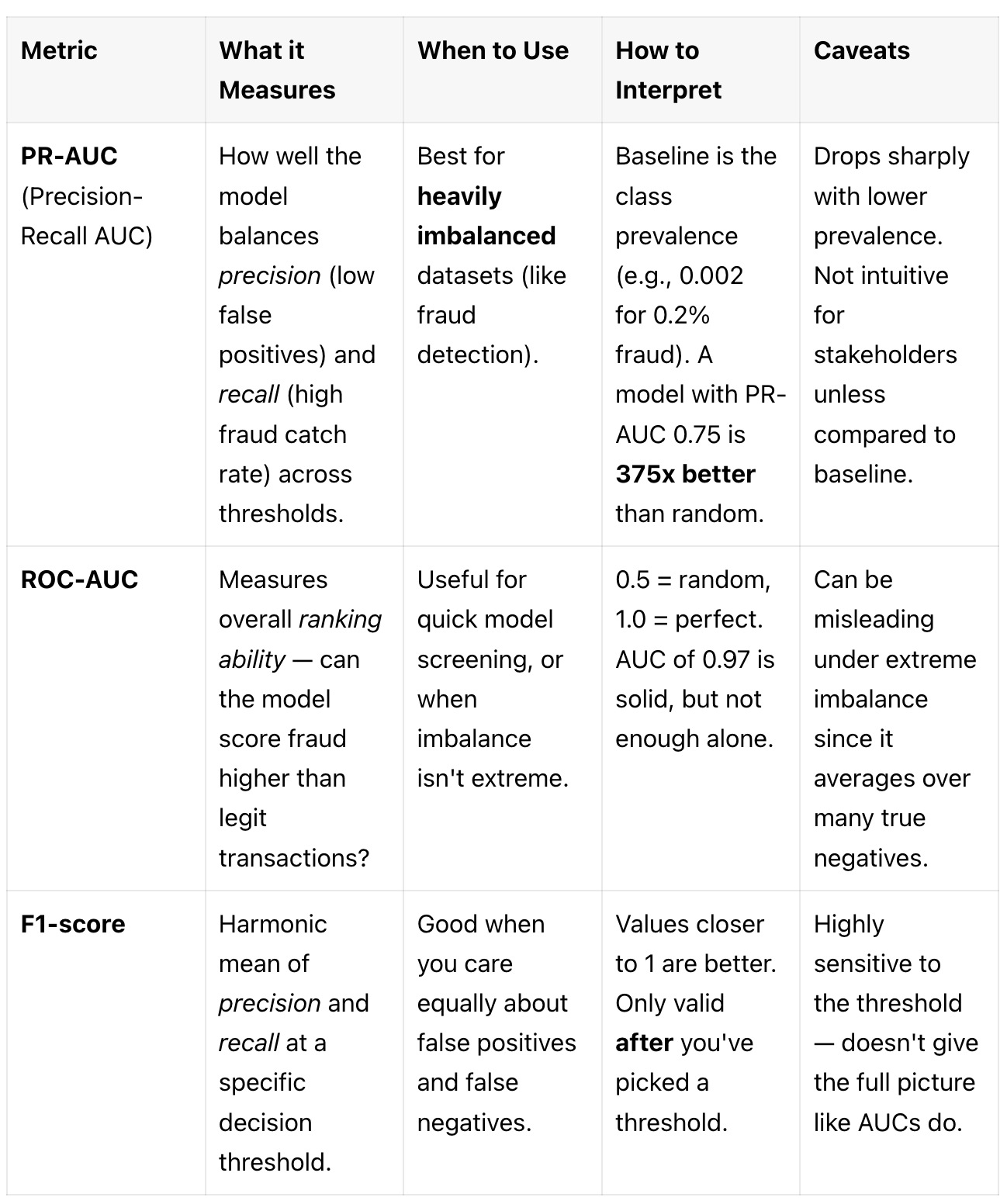
Rule of thumb: If positives ≪ negatives, prioritise PR-AUC for model selection and report confusion-matrix numbers at an operating threshold that meets business limits on false positives/negatives.

1. Downloads and loads the dataset

2. Performs exploratory data analysis (EDA)

3. Highlights correlations

4. Includes fraud ratio check, preprocessing, and baseline training

Code Lab: From Raw Fraud Data to First Model

Let’s go step-by-step through the credit card fraud dataset to see what imbalance really looks like—and how to start handling it.

Load the Data

You can download the data from here:

Then load it with pandas:

import pandas as pd

df = pd.read_csv("creditcard.csv")
print(df.shape)      
print(df["Class"].value_counts())

What we see:

• Legitimate transactions: 284315

• Fraudulent transactions: 492

• Fraud prevalence: 0.172% → classic ultra-imbalanced setup

Basic Preprocessing (Step-by-Step)

Before we train anything, we apply a few essential preprocessing steps to prepare the data.

Check for Missing Values

df.isnull().sum().any()

• df.isnull().sum() checks each column for how many missing (NaN) values it has.

• .any() returns True if any column has at least one null, otherwise False.

In our case, it returns False.

Scale the "Amount" Column

from sklearn.preprocessing import StandardScaler

scaler = StandardScaler()
df["Amount"] = scaler.fit_transform(df["Amount"].values.reshape(-1, 1))

Let’s break that down:

What's happening:

• StandardScaler() is a preprocessing tool that transforms values to have:

  • Mean = 0

  • Standard deviation = 1

Why do we scale Amount?

• Most of the features (V1 to V28) are already PCA-transformed (and thus standardized).

• But Amount is raw — it might range from very tiny values to several thousands.

• Without scaling, ML models like logistic regression or KNN might treat it as overly important just because of its larger scale.

Visual Correlation Scan

Let’s plot the correlation of all features with the Class (fraud).

import numpy as np
import matplotlib.pyplot as plt
import seaborn as sns

correlations = df.corr()["Class"].sort_values(ascending=False)

# Plot top and bottom features
plt.figure(figsize=(10, 6))
sns.barplot(x=correlations.values[:10], y=correlations.index[:10], palette="rocket")
plt.title("Top Positively Correlated Features with Fraud")
plt.show()

plt.figure(figsize=(10, 6))
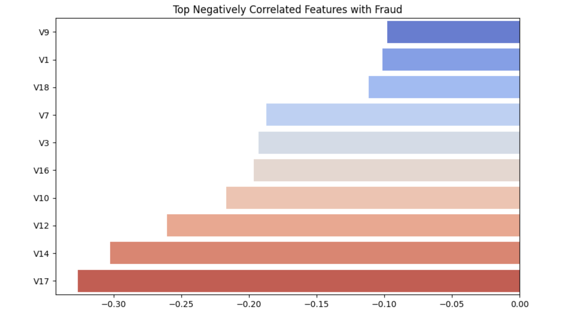
sns.barplot(x=correlations.values[-10:], y=correlations.index[-10:], palette="coolwarm")
plt.title("Top Negatively Correlated Features with Fraud")
plt.show()

Top Positively Correlated Features with Fraud

This plot shows which features have the strongest positive correlation with the fraud label (Class = 1).

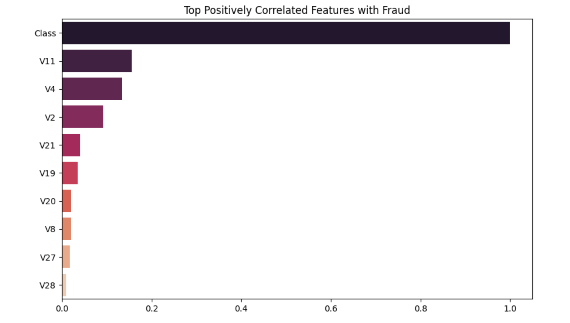
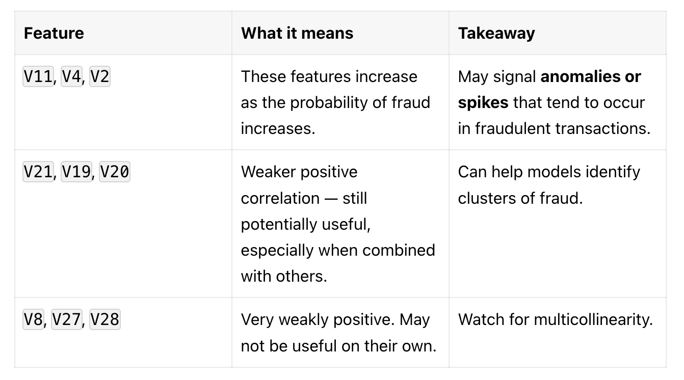
You can use these features as strong candidates in fraud risk scoring models, especially if you're building explainable systems.

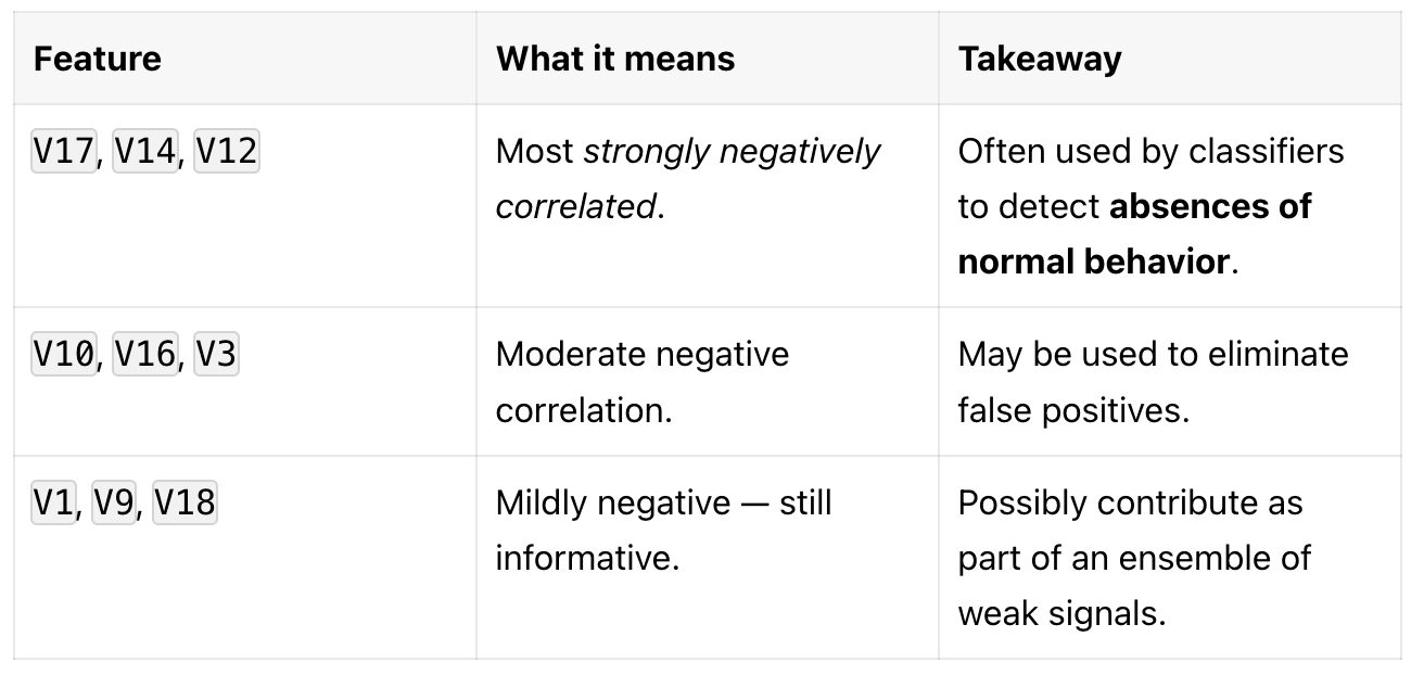
Top Negatively Correlated Features with Fraud

These features show a negative relationship with the fraud label — meaning their values tend to drop in fraud cases.

What to Do With This Info?

1. Feature Selection:

   • Prioritize features like V17, V14, V11, V4 when building lightweight or interpretable models.

   • Drop or regularize features with near-zero correlation (like V5, V6, V13) if using simpler models.

2. Multicollinearity Check:

   • Highly correlated features (e.g., V14 and V12) may introduce redundancy.

   • In linear models, drop or combine them. In tree models, it's less of an issue.

3. Model Insight:

   • Negative correlations often mean legitimate behavior is missing — a useful cue for anomaly detectors.

   • Positive correlations show fraud-specific patterns (e.g., outlier spikes or suspicious transactions).

Baseline Model Comparison: Naive vs. Balanced Approaches

To properly understand the impact of class imbalance, let's compare two approaches:

1. Naive Baseline: Standard logistic regression (ignores class imbalance)

2. Improved Baseline: Weighted logistic regression (accounts for class imbalance)

This comparison will show exactly why handling imbalance is crucial for fraud detection.

1. Imports & Stratified Data Split

from sklearn.model_selection import train_test_split
from sklearn.linear_model import LogisticRegression
from sklearn.metrics import (
    classification_report,
    average_precision_score,
    precision_recall_curve,
    confusion_matrix
)

import matplotlib.pyplot as plt
import seaborn as sns

We import train_test_split, LogisticRegression, average_precision_score, precision_recall_curve, and classification_report — all essential for training and evaluating models on imbalanced data.

# Define features and labels
X = df.drop("Class", axis=1)  # All features except target
y = df["Class"]               # Target: 0 = normal, 1 = fraud

We're splitting features and target. The Class column is the binary fraud label.

# Stratified split ensures class ratios are preserved
X_train, X_val, y_train, y_val = train_test_split(
    X, y, test_size=0.2, stratify=y, random_state=42
)

Why use stratification?

• Fraud is rare (~0.17% of samples).

• If we use a random split, we might end up with 0 fraud cases in validation — useless for evaluation.

• stratify=y keeps the same class ratio in both training and validation.

2. Train Naive Baseline (Standard Logistic Regression)

First, let's see what happens with a standard logistic regression that doesn't account for class imbalance:

# Naive baseline - standard logistic regression
naive_clf = LogisticRegression(
    max_iter=1000, 
    solver='liblinear'
)

naive_clf.fit(X_train, y_train)

# Predict probability scores and class labels
naive_proba = naive_clf.predict_proba(X_val)[:, 1]
naive_preds = naive_clf.predict(X_val)

# Evaluate naive baseline
naive_pr_auc = average_precision_score(y_val, naive_proba)
print("=== NAIVE BASELINE RESULTS ===")
print("PR-AUC Score:", round(naive_pr_auc, 4))
print("\nClassification Report:")
print(classification_report(y_val, naive_preds, digits=4))

# Confusion Matrix for naive baseline
naive_cm = confusion_matrix(y_val, naive_preds)
plt.figure(figsize=(6, 4))
sns.heatmap(naive_cm, annot=True, fmt="d", cmap="Blues")
plt.title("Naive Baseline - Confusion Matrix")
plt.xlabel("Predicted")
plt.ylabel("Actual")
plt.show()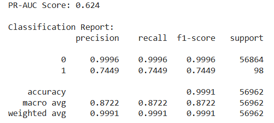

The naive baseline results perfectly illustrate why accuracy is misleading for imbalanced datasets:

The Deceptive Good News:

• High Accuracy (99.91%): Looks impressive but is meaningless

• High Precision for Legitimate Transactions (99.96%): Excellent at identifying normal transactions

• PR-AUC of 0.624: Actually not terrible, but we can do much better

The Critical Problems:

Terrible Fraud Detection Performance:

• Recall for Fraud: 74.49% - Missing 1 in 4 fraudulent transactions

• Only 73 out of 98 frauds caught - 25 frauds completely missed

• In fraud detection, missing 25% of fraudulent transactions is catastrophic

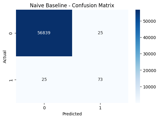
Confusion Matrix Reality Check:

• True Positives: 73 (frauds correctly identified)

• False Negatives: 25 (frauds missed - the worst outcome)

• False Positives: 25 (legitimate transactions flagged as fraud)

Why This Happens: The naive model is severely biased toward the majority class. With 99.83% of transactions being legitimate, the model learns that predicting "legitimate" is usually correct. It doesn't adequately learn the patterns that distinguish fraud.

Business Impact: In a real-world scenario, this means:

• Thousands in undetected fraud from those 25 missed cases

• Customer complaints from 25 false alarms

• Regulatory issues from inadequate fraud prevention

This demonstrates exactly why class balancing is essential for fraud detection.

3. Train Improved Baseline (Balanced Logistic Regression)

Now let's see how much better we can do by simply accounting for class imbalance:

clf = LogisticRegression(
    max_iter=1000, 
    class_weight='balanced', 
    solver='liblinear' # Works well for small to medium datasets
)

clf.fit(X_train, y_train)

class_weight='balanced' is key here.

• It tells the model to upweight fraud cases since they’re rare.

• Instead of sampling the data, we teach the model to care more about correctly predicting minority samples during training.

# Predict probability scores and class labels

proba = clf.predict_proba(X_val)[:, 1]  # Probability of being fraud
preds = clf.predict(X_val)              # Binary prediction: fraud or not

We keep both:

• proba for threshold-tuned evaluations (like PR curve)

• preds for default threshold (0.5) performance

4. Compare Results

# Compute PR-AUC for improved baseline
balanced_pr_auc = average_precision_score(y_val, balanced_proba)
print("=== IMPROVED BASELINE RESULTS ===")
print("PR-AUC Score:", round(balanced_pr_auc, 4))
print(f"Improvement over naive: {balanced_pr_auc/naive_pr_auc:.2f}x better")

# Detailed performance report
print("\nClassification Report:")
print(classification_report(y_val, balanced_preds, digits=4))

# Confusion Matrix Visualization
balanced_cm = confusion_matrix(y_val, balanced_preds)

fig, (ax1, ax2) = plt.subplots(1, 2, figsize=(12, 4))

sns.heatmap(naive_cm, annot=True, fmt="d", cmap="Blues", ax=ax1)
ax1.set_title("Naive Baseline")
ax1.set_xlabel("Predicted")
ax1.set_ylabel("Actual")

sns.heatmap(balanced_cm, annot=True, fmt="d", cmap="rocket", ax=ax2)
ax2.set_title("Improved Baseline (Balanced)")
ax2.set_xlabel("Predicted")
ax2.set_ylabel("Actual")

plt.tight_layout()
plt.show()

PR-AUC is much better than accuracy for imbalanced problems.

• It measures how well the model ranks frauds higher than non-frauds.

  

# Detailed performance report
print(classification_report(y_val, preds, digits=4))

This gives precision, recall, and F1-score per class, so you see how well fraud cases (Class 1) are being handled.

# Confusion Matrix Visualization
cm = confusion_matrix(y_val, preds)

sns.heatmap(cm, annot=True, fmt="d", cmap="rocket")
plt.title("Confusion Matrix")
plt.xlabel("Predicted")
plt.ylabel("Actual")
plt.show()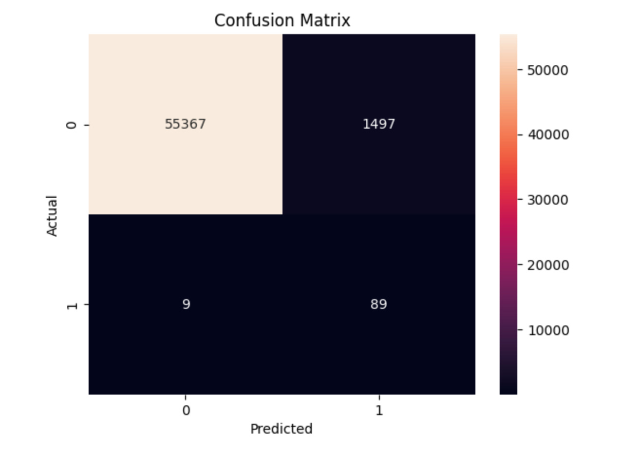

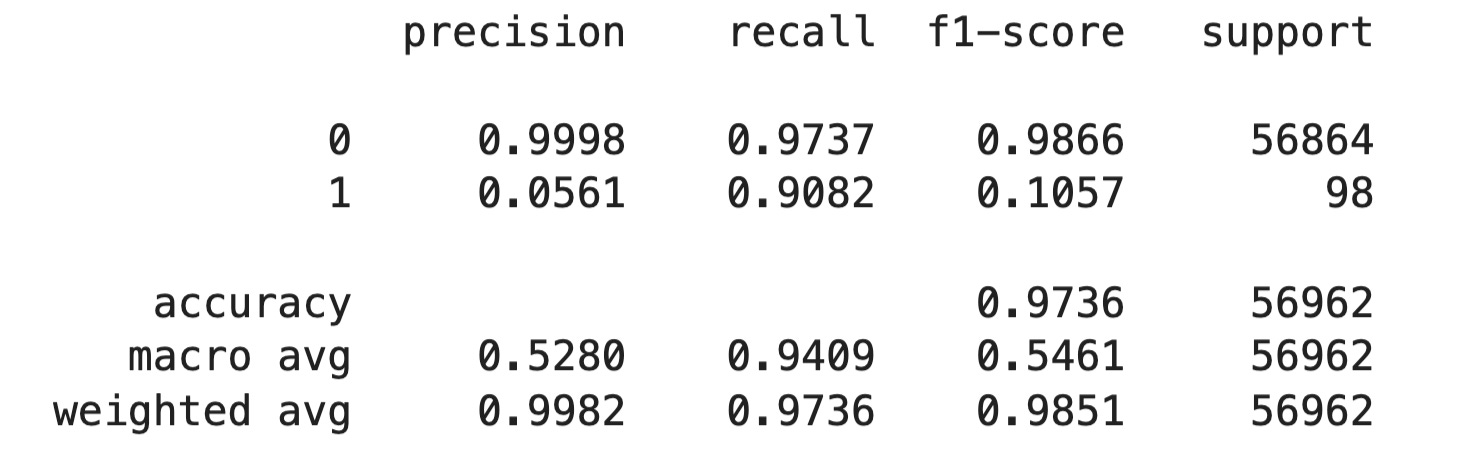
Key Difference in Results:

The improved baseline shows:

• True Negatives (TN): 55,367 → Non-fraud predicted correctly.

• False Positives (FP): 1,497 → Legit transactions wrongly flagged as fraud.

• False Negatives (FN): 9 → Fraud cases missed.

• True Positives (TP): 89 → Actual frauds correctly detected.

This shows a solid trade-off: we’re catching 91% of all frauds, with some cost in false alarms. A big jump from our baseline (which caught 0 frauds).

🎫 Machine Learning Summit 2025

Machine Learning Summit 2025 is where GenAI, LLMs, and ML systems meet the real world.

• 3 days

• 20+ expert speakers

• 100% focused on building and scaling practical AI solutions.

🗓️ When: July 16–18 (Online)

Key Tracks:

• Agents & GenAI in Action – From graph RAG to multimodal agents

• Applied ML & Model Performance – Interpretable, tabular-first, and time-aware models

• Production-Ready ML Systems – MLOps, observability, and scaling live systems

Featuring:
Anthony Alcaraz • Imran Ahmad • Kush Varshney • Andrea Gioia • Tivadar Danka and more

🎟️ Use code DAVID40 for 40% off

---

4. Visualize Precision–Recall Curve