


💊 Pill of the Week
Today we continue the Real World section. We walk through the full life cycle of a Customer Lifetime Value (LTV) prediction project, using the same telecom company from RW #1.

Customer Lifetime Value, or LTV, is the total value a customer is expected to generate for a business over a defined period, after accounting for revenue, upgrades, discounts, promotions, and other relevant costs. In this issue, we focus on predicting 24-month LTV for newly acquired telecom customers.
In RW #1 we built a churn model that identified which customers were about to leave. That solved a defensive problem. LTV prediction solves an offensive one: not just “who will we lose?” but “who is actually worth the most to us, and how do we invest accordingly?”
The same telecom now wants to answer a harder question. They spend millions every year acquiring new customers across paid search, TV advertising, retail stores, and online campaigns. Some of those customers stay for a decade and upgrade multiple times. Others churn after two months having never paid full price. Right now, the acquisition team treats them identically. The goal of this project is to change that.
For a refresher on each phase of the data science lifecycle without focusing on this concrete example, check the previous issues:
In this issue, we walk through the full lifecycle of a Customer Lifetime Value (LTV) prediction project for a telecom company:
How to define the LTV problem and agree the business objective
What data is needed to predict 24-month customer value
How to clean the data and avoid leakage
How exploratory analysis reveals early value signals
Which features matter most by day 60
How to choose the right modelling approach
How to train the model using cohort-based splits
💎How to evaluate performance with technical and business metrics
💎How to refine the model through better features and calibration
💎How to deploy LTV predictions into production
💎How to communicate the results to stakeholders
💎How to monitor the model after launch
The goal is to show how early customer behaviour can help predict long-term value, so acquisition and retention budgets are invested where they are most likely to pay off.
Let’s start!
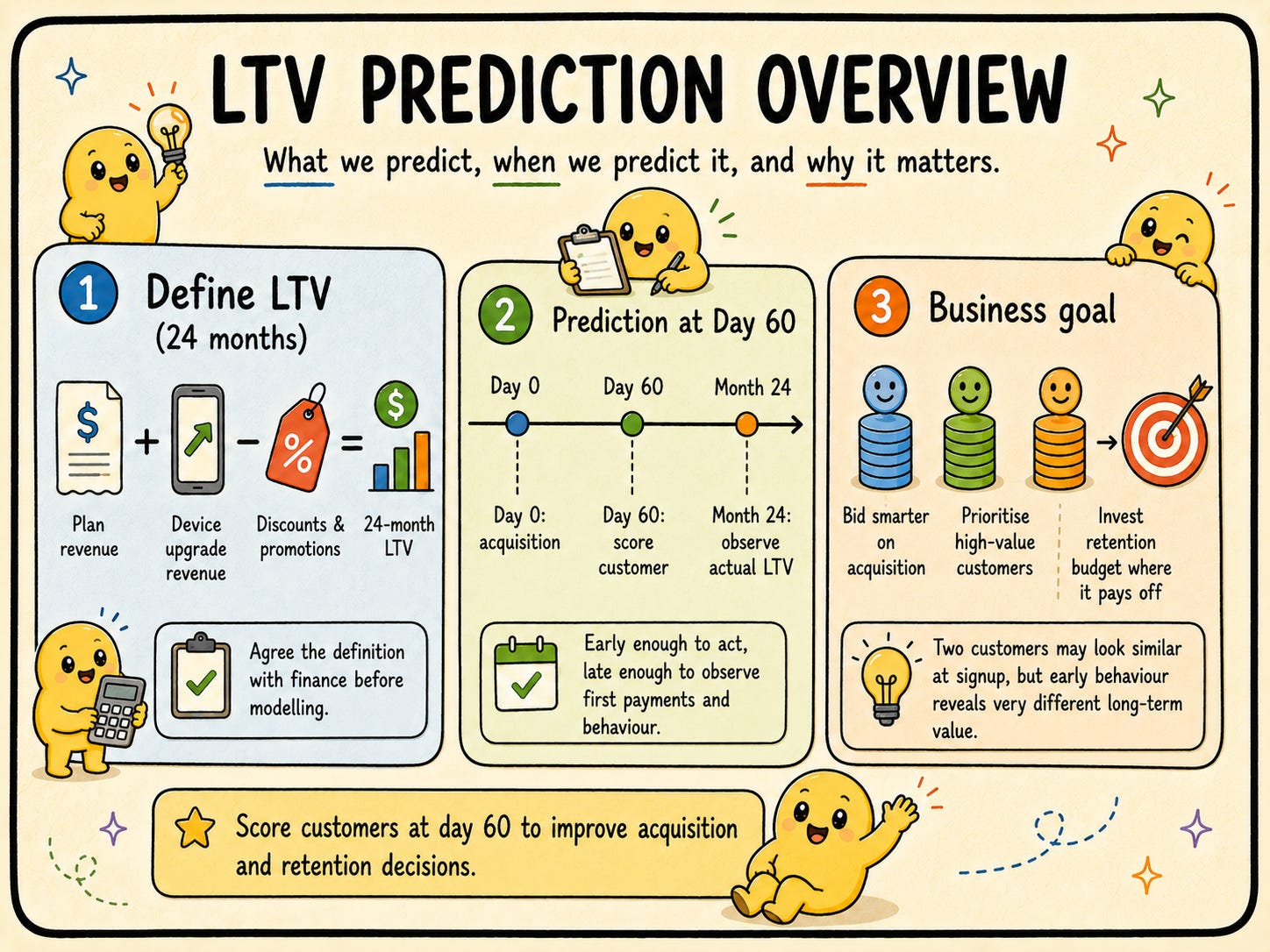
1. Define the Problem or Question to be Answered
Objective: Predict the 24-month LTV of newly acquired customers within their first 60 days, with enough accuracy to adjust acquisition channel bids and prioritize retention investment on high-value segments.
Problem Statement: “Which newly acquired customers will generate the most revenue over the next two years, and how can we use that prediction to stop wasting acquisition budget on customers who will never be profitable?”
Key Considerations:
LTV Definition: The telecom defines LTV as total plan revenue plus device upgrade revenue, minus discount and promotion costs, over a 24-month window. Crucially, this must be agreed with the finance team before a single line of code is written. Different definitions produce different models with different business implications.
Time Horizon: 24 months fits the telecom contract cycle. A customer on a 24-month handset contract has a natural LTV floor set by the contract value, which gives the model a useful lower bound.
Prediction Trigger: The team scores customers at day 60. Early enough to act, late enough to observe first bill payment, whether the customer upgraded their plan, and whether they contacted support.
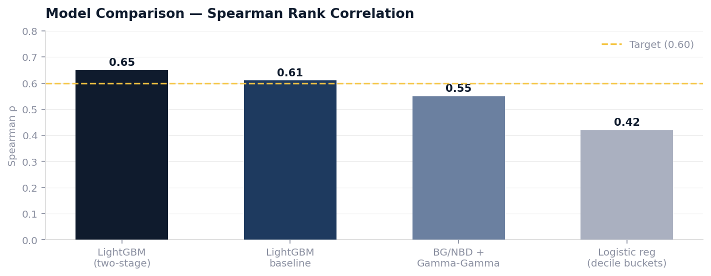
KPIs: The primary success metric is Spearman rank correlation between predicted and actual LTV at the 24-month mark. The business metric is improvement in average LTV per acquisition pound spent, measured six months after deployment.
Example: A customer acquired through a TV campaign who activates a family plan within the first 30 days and pays the first two bills on time is a very different prospect than a customer acquired through a price comparison site who immediately calls to complain about the activation fee. Both entered the same acquisition funnel. LTV prediction separates them.
2. Gather and Understand the Data
Data Collection:
Internal Sources: CRM records, billing system exports, plan and tariff data, customer support call logs, device upgrade history, payment success and failure records, promotional discount history.
External Sources: Network quality scores by postcode (signal strength, outage frequency), Ofcom churn benchmarks by region, competitor pricing snapshots.
Data Understanding:
Data Inventory: List every feature available at the day 60 prediction trigger. First bill status, number of support calls in the first 60 days, whether the customer opted into auto-renewal, plan tier (SIM-only vs handset vs family), acquisition channel, and promotional offer used at signup.
Target Variable: Compute actual 24-month LTV for all customers acquired in the previous three years who have now reached their 24-month mark. This is the training set.
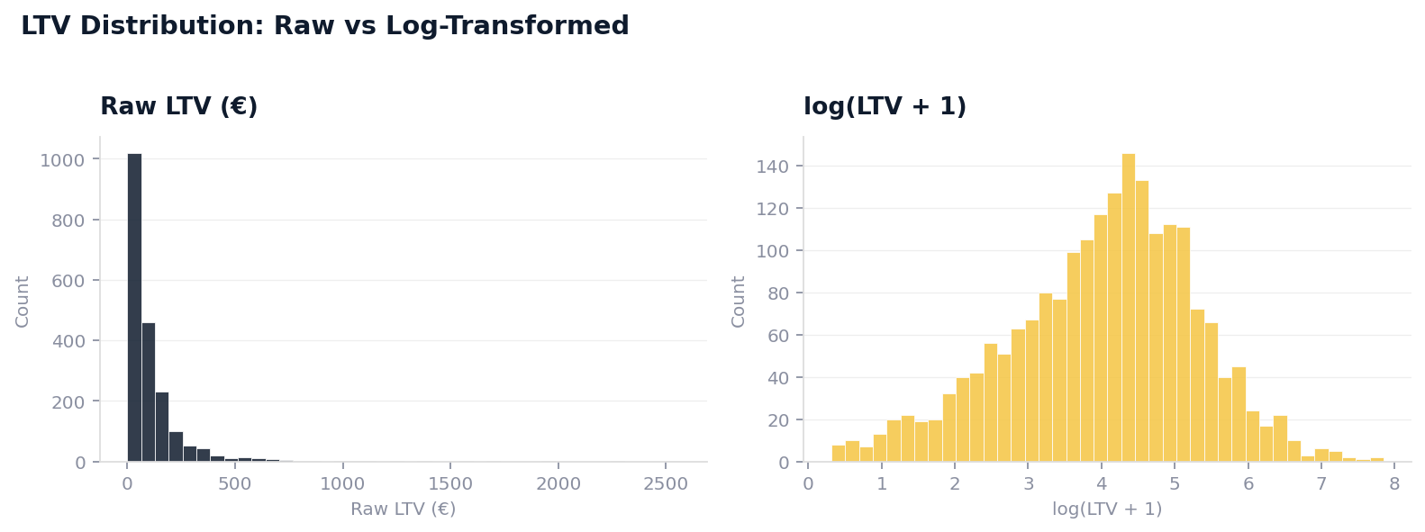
Data Quality Assessment: LTV is right-skewed. The majority of customers cluster around the contract minimum value. A small tail of family plan customers with multiple upgrades drives a disproportionate share of total revenue.
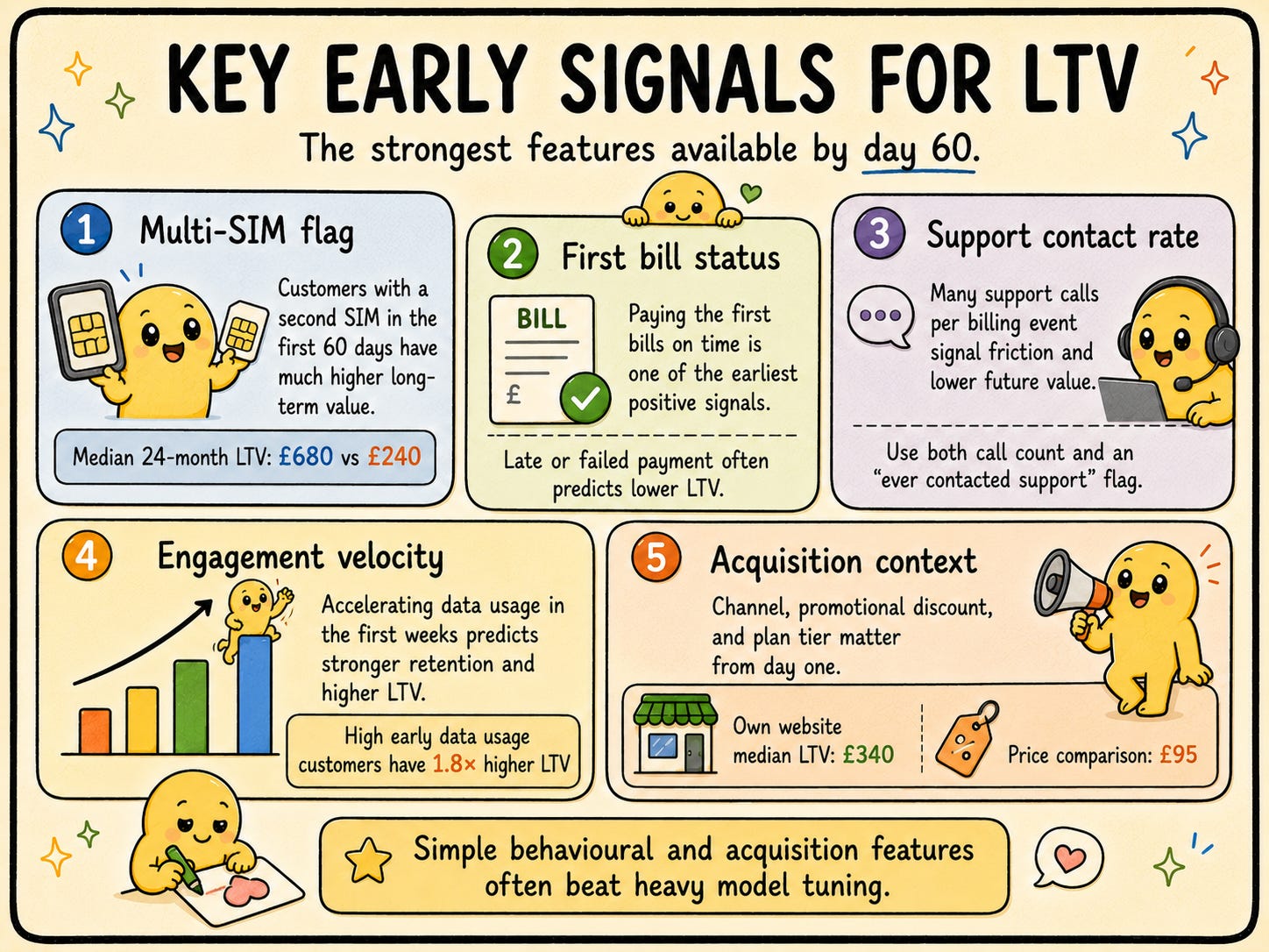
Example Insight: Customers who activate a second SIM within the first 60 days (suggesting a family or shared plan) have a median 24-month LTV of £680, versus £240 for single-SIM customers acquired in the same month. This single variable becomes one of the strongest predictors in the model.
3. Prepare and Clean the Data
Data Cleaning Steps:
Handle Missing Values: Support call count is null for customers who never called, not missing at random. Replace null with zero and add a binary “ever contacted support in 60 days” flag to preserve the signal.
Remove Leakage: This is the single most important step. Every feature must have been observable at day 60. Plan upgrade revenue at month 18 cannot be used. Payment history at day 45 can be. The team reviews every column against a strict cutoff calendar.
Winsorize the Target: Cap LTV at the 99th percentile (£2,400 in this dataset) during training. The handful of enterprise accounts above that level are handled by the B2B team and are not relevant to the consumer acquisition model.
Cohort-Based Splits: Train on customers acquired in months 1 to 24, validate on months 25 to 30, test on months 31 to 36. Never use random train-test splits on this data. A customer acquired in January 2022 and one acquired in January 2024 lived through different network quality levels, pricing environments, and competitor landscapes.
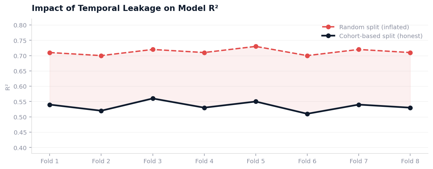
Example: When the team first trains without cohort-based splitting, the validation R² is 0.71. Switching to temporal splits drops it to 0.54. The team initially sees this as a problem. It is not. 0.54 is the honest number. 0.71 was a flattering lie caused by the model memorizing future patterns.
4. Perform Exploratory Data Analysis (EDA)
EDA Techniques:
Target Distribution: Confirm log(LTV + 1) is approximately normal. Plot separately for contract type (SIM-only, handset, family) because the distributions are structurally different and may warrant separate models.
Cohort Analysis: Compare LTV distributions by acquisition year and by acquisition channel. If the 2022 cohort and the 2024 cohort look very different, that is not noise, it is a signal that the model should weight recent cohorts more heavily.
Feature-Target Relationships: Plot the 10 most correlated features against log LTV. Expect non-linear relationships for variables like days to first bill payment (customers who pay on day 1 are very different from those who pay on day 28).
Correlation Analysis: Build a correlation matrix. In this dataset, total plan spend in 60 days and plan tier are highly correlated. Keep plan tier because it is more interpretable and has lower variance.
Insights:
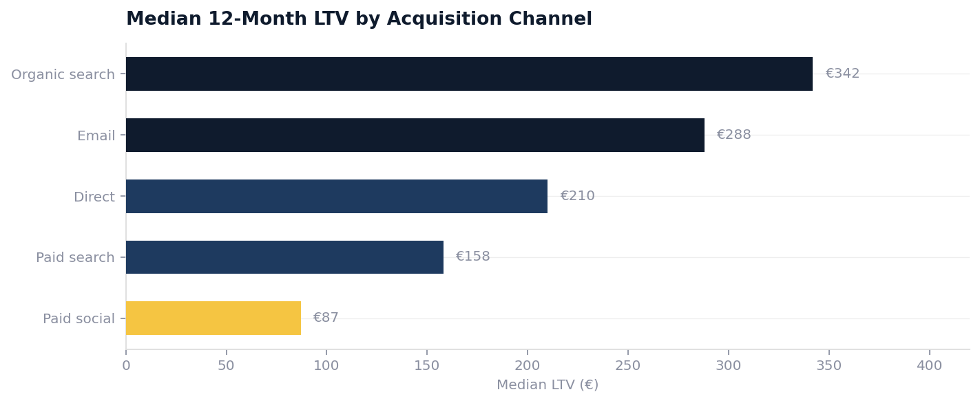
Channel Gap: Customers acquired through the operator’s own website have a median LTV of £340, versus £95 for customers acquired through price comparison sites. The price comparison channel drives volume but destroys margin.
Early Behavior as Signal: Customers who use mobile data above the median in their first 30 days are 60% less likely to churn and have 1.8x higher LTV. High data usage signals genuine engagement with the service.
Example: EDA reveals that postcode-level network quality score interacts strongly with plan tier. High-value customers on premium plans in areas with poor signal have LTV 35% lower than equivalent customers in good-coverage areas. This becomes an important interaction feature.
5. Engineer Relevant Features
Feature Engineering:
RFM at Day 60: Recency (days since last top-up or bill payment), Frequency (number of billing events), Monetary (total plan charges paid). These three features alone beat most naive baselines.
Engagement Velocity: Week-over-week change in data usage from week 1 to week 8. Customers whose usage is accelerating have higher LTV than customers whose usage is flat or declining, even if absolute usage levels are similar.
Multi-SIM Flag: Binary indicator for whether the account has more than one active SIM at day 60. The single highest-lift binary feature in the dataset.
Support Contact Rate: Number of support calls divided by number of billing events. High ratios signal friction that predicts churn and lower LTV.
Network Quality at Signup Postcode: Median download speed and outage frequency for the customer’s home postcode, joined from network operations data. Customers in poor-coverage areas have systematically lower LTV regardless of their plan tier.
Acquisition Context: Channel (own website, retail store, price comparison, TV campaign), promotional offer depth (percentage discount at signup), and device category (premium handset, mid-range handset, SIM-only).
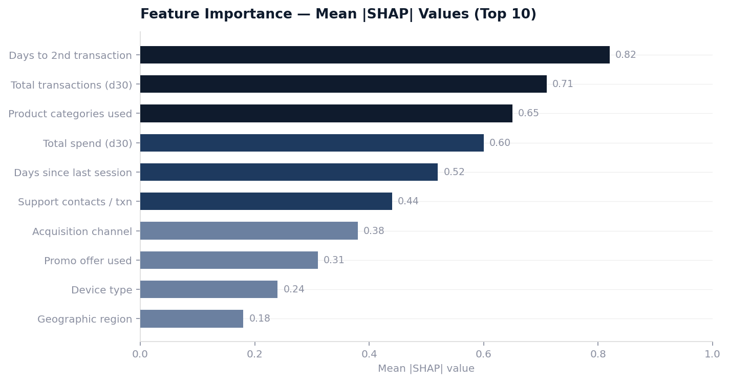
Example Feature: Days between activation and first data usage above 1GB is a compact but highly predictive feature. Customers who hit that threshold within the first 7 days show consistently higher 24-month LTV across all acquisition channels and plan tiers.
6. Select Appropriate Modeling Techniques
Modeling Approaches:
Regression on Log-Transformed Target: Predict log(LTV + 1) and exponentiate predictions. This is the baseline. Simple, fast to train, and produces a calibrated output that finance can work with.
BG/NBD + Gamma-Gamma: The Buy-Till-You-Die probabilistic model family is a strong benchmark when transaction-level data is available. For telecoms with regular billing events, this model decomposes LTV into expected number of billing cycles times expected spend per cycle. Very interpretable for actuarial conversations with the finance team.
LightGBM on Log-Transformed Target: Handles non-linearities and interaction terms between features like plan tier and network quality without manual specification. In this dataset it outperforms linear models significantly once the engagement velocity and network quality features are included.
Two-Stage Model: Stage 1 classifies customers into “active at 24 months” vs “churned before 24 months” (leveraging the churn model from RW #1). Stage 2 predicts revenue conditional on staying active. This mirrors the probabilistic model structure and produces better-calibrated estimates at the high end.
Chosen Model: LightGBM on log-transformed LTV, with the two-stage variant used for the top decile where prediction accuracy matters most for premium acquisition bidding.
Example: The churn model from RW #1 becomes a direct input into Stage 1 of the LTV model. Customers with a high predicted churn probability in the first 6 months are assigned lower LTV estimates regardless of their early spending behavior. Two projects that were developed separately now work together.
7. Train the Models Using the Prepared Data
Training Process:
Data Splitting: Train on acquisition cohorts from months 1 to 24, validate on months 25 to 30, test on months 31 to 36. All splits are by cohort month, not by individual customer.
Target Encoding: Acquisition channel and postcode district are high-cardinality categoricals. Encode them with out-of-fold target encoding to avoid leakage within the training set.
Stage 1 Class Imbalance: High-value customers (top 20% of LTV) represent a small fraction of the training data. Apply class weights in Stage 1 classification to improve sensitivity for the segment where prediction errors are most expensive.
Walk-Forward Validation: Run 8 walk-forward validation windows, each training on the data available up to that point and evaluating on the next two months of cohorts. This simulates exactly how the model will behave in production.
Tracking:
Log all experiments in MLflow, recording features used, hyperparameters, cohort window definition, and validation metrics. The team runs 47 experiments before settling on the final configuration.
Monitor residuals by acquisition channel separately. The model has systematically higher errors for TV campaign customers early in the experiment runs, which turns out to be explained by a missing interaction between promotional depth and plan tier.
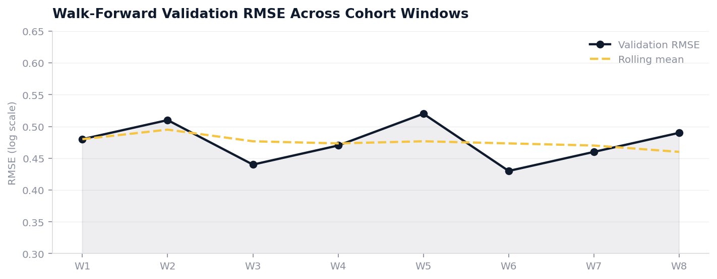
Example: The model trained without walk-forward validation shows stable RMSE on a single held-out cohort. Switching to 8 walk-forward windows reveals that RMSE is higher on the two most recent cohorts, driven by a pricing change that made SIM-only plans cheaper. The team adds a “SIM-only flag times acquisition year” interaction feature that resolves the issue.
8. Evaluate the Model’s Performance
Keep reading with a 7-day free trial
Subscribe to Machine Learning Pills to keep reading this post and get 7 days of free access to the full post archives.