RW #6 - Text-Moderation System with Embeddings

💊 Pill of the Week

This week we’re handing you a plug-and-play, notebook-ready tutorial you can drop straight into Jupyter or VS Code. Inside you’ll find:

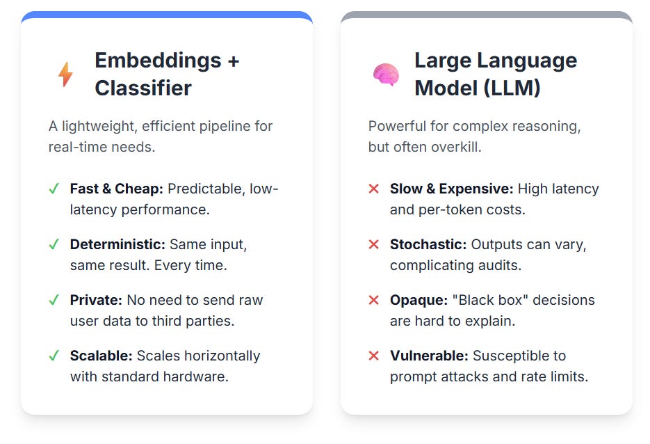
• Why an embedding-plus-classifier pipeline trumps funneling every chat message through a giant LLM—think millisecond latency, predictable cost, and rock-solid determinism.

• A cell-by-cell build of that pipeline, with plain-English commentary before and after each code block so you always know what you’re running and why it matters.

By the end you’ll walk away with production-grade moderation code you can ship as-is—or adapt to your own data in minutes.

Why choose an embeddings-based classifier?

When a sentence is converted into a dense vector, texts that share meaning land near one another even if the wording differs. Training a lightweight classifier on those vectors brings five practical gains:

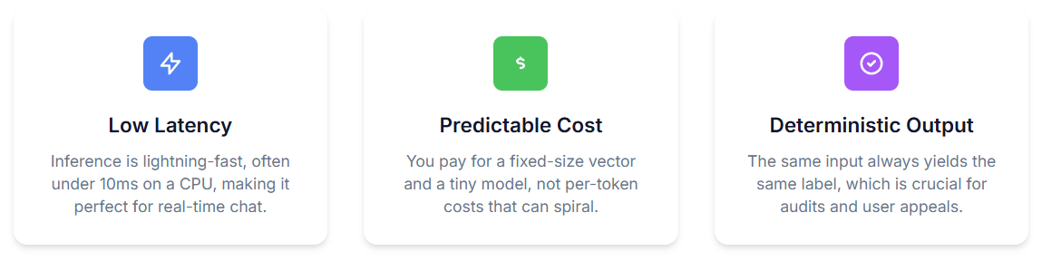
1. Low latency – inference often completes in under ten milliseconds on a CPU.

2. Predictable cost – you pay only for a fixed-size vector and a tiny model, not per token.

3. Wide language coverage – modern encoders such as MiniLM or LaBSE generalise well across dozens of languages.

4. Deterministic output – the same input always yields the same label, simplifying appeals.

5. Easy retraining – a fresh batch of labelled messages and one fit command are all that is needed when policy changes.

Why sending every message to an LLM is often overkill

LLMs excel at reasoning over long passages, yet they come with seven drawbacks that matter in real deployments:

• Cost and throughput: token-priced calls and GPU reliance make per-message moderation expensive at scale.

• Latency: even small hosted models usually take hundreds of milliseconds, which users notice in live chat.

• Stochasticity: identical prompts can give different judgements later, complicating audits.

• Opaque decisions: explaining a multi-billion-parameter model to regulators is far harder than pointing to a logistic coefficient and a nearest-neighbour example.

• Prompt attacks: adversaries can hide violations behind role-play or system-message tricks; a pure classifier ignores prompts altogether.

• Privacy concerns: shipping every raw message to a third-party endpoint may breach GDPR or internal policy, whereas local embeddings avoid this.

• Rate limits and outages: hosted LLMs throttle traffic; a self-hosted embedding pipeline scales horizontally on standard hardware.

LLMs are still useful for low-volume, long-form reviews or as a second pass on borderline cases, but for a busy chat stream an embedding pipeline wins on speed, cost and predictability.

Hands-on example

Here we aim to demonstrate how to build a highly efficient and reliable text moderation system for high-volume applications, such as live chat.

We achieve this by using a lightweight, two-part pipeline:

1. converting text messages into numerical sentence embeddings

2. training a small, fast classifier on those embeddings

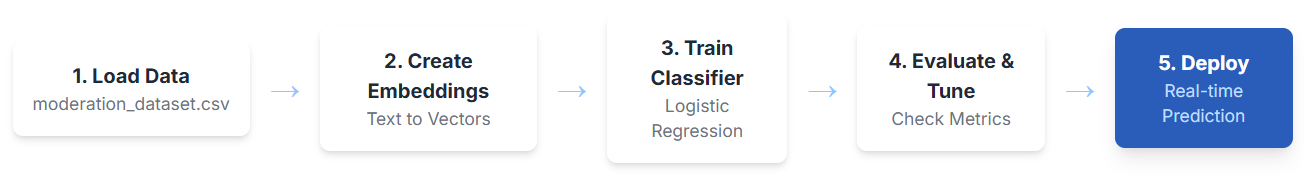
This method is designed to be superior to using a large language model (LLM) for every message, as it provides extremely low latency, predictable and low costs, and deterministic outputs that are easy to audit and scale.

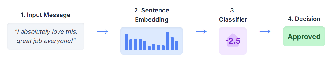
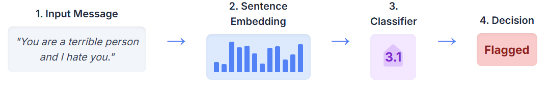
The following simple flowcharts illustrate how the pipeline processes and flags a message. A message is converted into a vector, scored by the classifier, and then a final decision is made based on the score.

• Valid input message:

• Input message that must be moderated:

Let’s begin with the real-world coding example:

Environment set-up

Install the required libraries. Skip this cell if your environment already has them.

!pip install -q sentence-transformers scikit-learn pandas matplotlib

Import core modules

We import everything the notebook will need.

from sentence_transformers import SentenceTransformer
from sklearn.model_selection import train_test_split
from sklearn.linear_model import LogisticRegression
from sklearn.metrics import classification_report, RocCurveDisplay
import pandas as pd
import matplotlib.pyplot as plt

Load and inspect data

Our dataset, moderation_dataset.csv, contains two columns:

• text: the message content

• label: a binary flag where 1 indicates the message requires moderation, and 0 means it is acceptable.

df = pd.read_csv("moderation_dataset.csv")
df.head(15)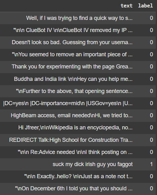

For this example we’ve used data from this Kaggle competition:

Let’s check the label distribution:

df.label.value_counts()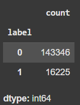

Our dataset is highly imbalanced, though it includes a large number of minority class examples. In this example, we'll apply balanced sampling to train on an even class distribution. Also, we will take only 1000 sentences for this example, but more can be used to improve accuracy.

df = pd.concat((
    df[df.label == 1].sample(500),
    df[df.label == 0].sample(500)
), axis=0)

Alternatively, we could keep the natural imbalance and compensate using class weights—particularly useful when resampling isn't desirable or leads to overfitting.

Create sentence embeddings

We will use OpenAI’s text-embedding-3-small model with 256 dimensions. This offers high-quality multilingual embeddings in a compact size suitable for low-latency tasks.

from openai import OpenAI
from tqdm import tqdm

client = OpenAI(api_key=OPENAI_API_KEY)

embeddings = []
for text in tqdm(df["text"].tolist(), desc="Embedding texts"):
    response = client.embeddings.create(
        input=text,
        model="text-embedding-3-small",
        dimensions=256
    )
    embeddings.append(response.data[0].embedding)

Make sure the OPENAI_API_KEY is set in your environment beforehand. The 256-dimensional variant strikes a good balance between quality and performance for classification tasks.

Prepare train and test sets

A stratified split keeps the class ratio consistent.

X_train, X_test, y_train, y_test = train_test_split(
    embeddings,
    df["label"],
    test_size=0.20,
    stratify=df["label"],
    random_state=42
)

Using a fixed random seed makes results reproducible.

---

📖 Book of the Week

Ready to pair large-language-model magic with the power of knowledge graphs?

Today I share with you “Building Neo4j-Powered Applications with LLMs”

Ravindranatha Anthapu and Siddhant Agarwal’s brand-new guide shows—step by step—how to stand up a full Retrieval-Augmented Generation (RAG) stack on Neo4j, then ship it to production on Google Cloud.

Why it’s worth your coffee break?

• Hands-on RAG pipeline: ingest, summarize, embed, and retrieve customer behavior data with LangChain4j, then wire it all together in Spring AI.

• Graph + vector search that just works: blend Cypher queries with Haystack’s hybrid retrieval to serve smarter, context-rich answers.

• Less hallucination, more reasoning: grounding techniques and multi-hop patterns that keep LLMs honest.

• Deploy in one push: opinionated blueprint for CI/CD to GCP—including secrets, auth, and cost tips.

You can get it here:

---

Train a baseline classifier

Logistic regression handles dense embeddings well and trains in seconds.

clf = LogisticRegression(
    max_iter=200,
    class_weight="balanced"  # helps if classes are uneven
)
clf.fit(X_train, y_train)

Here we are using class_weight="balanced" in addition to the balanced sampling to handle imbalanced data. This method is often a superior and more robust method for production use cases as it adjusts the loss function without throwing away data.

Evaluate initial performance

We first look at metrics using the default 0.5 threshold.

y_pred = clf.predict(X_test)
print(classification_report(y_test, y_pred, digits=3))

The result is:

              precision    recall  f1-score   support

           0      0.885     0.850     0.867       100
           1      0.856     0.890     0.873       100

    accuracy                          0.870       200
   macro avg      0.871     0.870     0.870       200
weighted avg      0.871     0.870     0.870       200

The model demonstrates a well-balanced performance across both classes, with an overall accuracy of 87%. Unlike in more imbalanced scenarios, here the dataset is evenly split between toxic and non-toxic examples, allowing for a more reliable assessment of the model’s behavior. The results show a strong and symmetric classification capability: for the non-toxic class, the model achieves a precision of 88.5% and a recall of 85.0%, while for the toxic class, it reaches a precision of 85.6% and a slightly higher recall of 89.0%.

The F1-scores for both classes are nearly identical—0.867 for non-toxic and 0.873 for toxic—indicating that the model handles both categories with comparable effectiveness. The macro and weighted averages are also closely aligned, further confirming the balance. These results suggest that the model is both accurate and fair in its predictions, capable of distinguishing between harmful and harmless content without favoring one class over the other. This kind of performance is especially promising for applications in content moderation, where both false positives and false negatives can carry significant consequences.

If your policy prioritises identifying as many violations as possible—even at the risk of flagging some false positives—then you should focus on optimising recall for the positive class. This approach ensures that the model is highly sensitive to potential infractions, catching almost every instance that might constitute a violation, which is particularly critical in contexts like fraud detection, content moderation, or safety compliance.