


Issue #62 - ARIMA model from zero to hero
Issue #62 - ARIMA model from zero to hero


💊 Pill of the week
Time series data, characterized by observations over sequential time intervals, often exhibits patterns and trends that can be analyzed and forecasted using sophisticated statistical models. One such powerful model is ARIMA (AutoRegressive Integrated Moving Average), which combines autoregressive (AR), differencing (I), and moving average (MA) components to capture the temporal dependencies within the data.
🛠️ DIY
In this article we will show how to train an ARIMA model. We will focus on the results and steps, without showing the code, since it was already introduced in previous issues of MLPills. However, we will share a notebook with all the code you need to train your ARIMA model at the end of the issue!
⚠️Notebook at the end of the issue ⚠️
Step 1: Loading the data and Understanding the process
To begin our analysis, we start by importing essential libraries like numpy and pandas, which facilitate numerical operations and data manipulation, respectively. Loading our time series data using pd.read_csv() allows us to set appropriate timestamps as the index, ensuring accurate time-based analysis.
You can also revise this issue in which we introduced the ARIMA model and its components:

We will follow the so-called Box-Jenkins method:

Step 2: Assessing Stationarity
Before applying ARIMA, it's crucial to ensure that our time series data is stationary. This will be allow us to determine the value of “d”. Stationarity implies that the statistical properties such as mean and variance remain constant over time, which is essential for modeling.
We employ two primary tests for stationarity:
Augmented Dickey-Fuller (ADF) Test: This test examines whether a unit root is present in the series. A lower p-value (< 0.05) from this test suggests that the series is stationary.
Kwiatkowski-Phillips-Schmidt-Shin (KPSS) Test: In contrast, this test checks for stationarity around a deterministic trend. A higher p-value (> 0.05) indicates stationarity.

In the example we observe that the initial data is not stationary, we could actually see if just by plotting the graph:
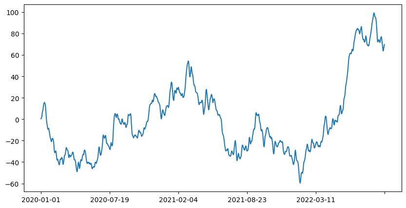
This means that we will need to difference the data, “d” won’t be 0.
Step 3: Preparing the Data - Differencing
The series is not stationary based on the initial tests, so we apply differencing. Differencing involves subtracting the previous observation from the current one, a process denoted by the parameter “d” in ARIMA. This transformation helps stabilize the mean and variance of the series.
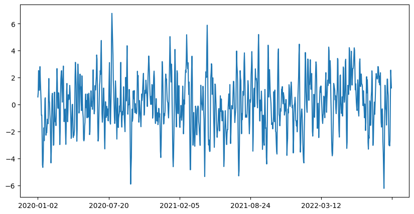
This looks way better!
If we perform the stationarity tests we get that it is stationary:
Augmented Dickey-Fuller (ADF) Test:
ADF Statistic: -8.770582534427128
p-value: 2.5274599738010693e-14
Critical Values:
	1%: -3.437
	5%: -2.864
	10%: -2.568
ADF test: Series is stationary
Kwiatkowski-Phillips-Schmidt-Shin (KPSS) Test:
KPSS Statistic: 0.19664101759123429
p-value: 0.1
Lags Used: 11
Critical Values:
	10%: 0.347
	5%: 0.463
	2.5%: 0.574
	1%: 0.739
KPSS test: Series is stationary
Since we had to differenciate once before making our data stationary, we know that the parameter d of the ARIMA model will be equal to 1.
We can proceed with the other two parameters: p and q.
Step 4: Visualizing Correlations - ACF and PACF
To determine the appropriate parameters p (AR) and q (MA) for our ARIMA model, we plot:
Autocorrelation Function (ACF): This plot shows the correlation between the series and its lagged values, aiding in identifying the MA order (
q).Partial Autocorrelation Function (PACF): This plot indicates the direct relationship between a lag and the series, helping to determine the AR order (
p).

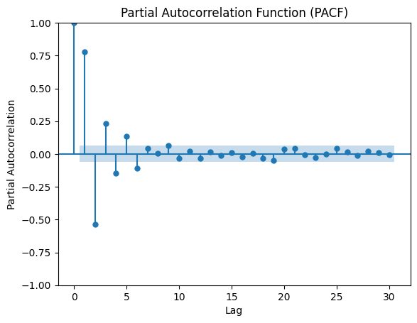
First we can check the ACF plot of the undifferenced data:
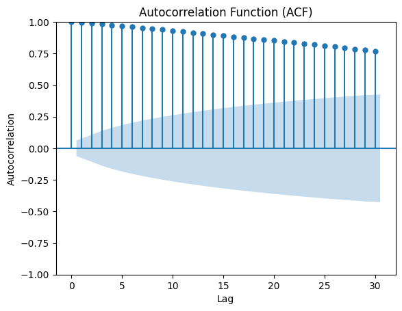
You can see that the ACF plot shows a slow decay, which indicates that differencing was indeed necessary.
Now let's plot the PACF and ACF of the differenced data (d=1) to see the difference:
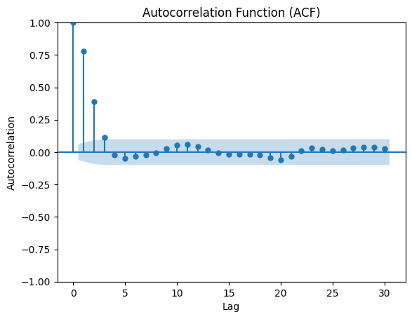
A sharp decline in autocorrelation is observed in both plots, which indicates stationarity, confirming that the selected d value (1) was appropriate.
This will also help us estimate the values for p and q:
The order of the AR term (p) is typically chosen based on the Partial Autocorrelation Function (PACF) plot, in this case: p = 6
The order of the MA term (q) is typically chosen based on the Autocorrelation Function (ACF) plot, in our case: q = 3
Step 5: Building and Refining the ARIMA Model
Armed with insights from the ACF and PACF plots, we construct our ARIMA model. Iteratively adjusting parameters based on model diagnostics such as AIC (Akaike Information Criterion) and BIC (Bayesian Information Criterion), we aim to find the best-fit model that minimizes these metrics.
We start by checking the model summary:
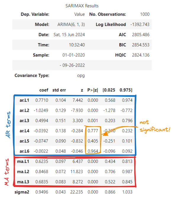
We observe that the AR terms 4 to 6 are not significant (p-value [P>|z|] < 0.05). So that may indicate that we've overestimated the value of p, let's reduce it to 4 and do the same again:
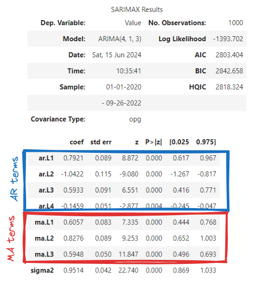
Now all terms are significant! Great! Let's compare the AIC and BIC to see if they are better (lower) too:
ARIMA(6,1,3) → AIC = 2805.486, BIC = 2854.553
ARIMA(4,1,3) → AIC = 2803.404, BIC = 2842.658
It is not a big change but the new model is better! We ideally should repeat this with several combinations of parameters (around our estimation and verifying that the AR and MA terms are significant) until we achieve the optimal AIC and BIC (the lowest).
Here an introduction to these concepts:

Step 6: Evaluating Model Performance
Once the ARIMA model is trained, we proceed to evaluate its performance:
Residual Analysis: We inspect the residuals to ensure they exhibit no discernible patterns, resembling white noise. Diagnostic checks like Q-Q plots and histogram of residuals verify this assumption.
Forecasting: Using the fitted model, we generate forecasts for future time points and compare them against actual values. Metrics such as MAE, RMSE, and others quantify the accuracy of our predictions.
In this issue we will focus solely on the first one, residual analysis, leaving the second one for a future issue.
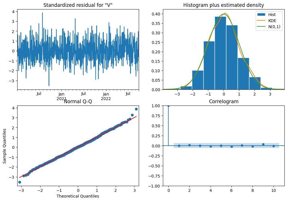
We observe:
No obvious patterns in the residuals → random noise
Histogram looks like a normal distribution
The majority of datapoints lie over the line in the normal Q-Q graph
All lags (apart from the 0) are within the confidence range (blue-shaded area).

Great news, our model is capturing the data!
In a future issue…
The next steps would be to assess the accuracy of the model:
Split your data: Set aside a portion of your data as a test set. Typically, this is done by holding out the last portion of your time series data. For example, you could use the last 20% of your data for testing and the first 80% for training.
Refit the model on the training data: Fit your ARIMA model using only the training data. This ensures that your model does not have knowledge of the future values that it is supposed to predict.
Forecast: Use your trained model to forecast the values for the period covered by the test set. Compare these forecasted values with the actual values in the test set.
Evaluate the forecast accuracy: Calculate accuracy metrics such as Mean Absolute Error (MAE), Mean Squared Error (MSE), Root Mean Squared Error (RMSE), and Mean Absolute Percentage Error (MAPE). These metrics will give you an indication of how well your model is performing.
Visualize the results: Plot your forecasted values against the actual values to visually inspect how well your model is capturing the trends and patterns in the data.

In conclusion, ARIMA stands as a robust methodology for analyzing and forecasting time series data, offering insights into trends and patterns that are invaluable for decision-making across various domains. By following these systematic steps, analysts and data scientists can leverage ARIMA to derive actionable insights and make informed predictions from time series data.
🎓Learn Real-World Machine Learning!*
Do you want to learn Real-World Machine Learning?
Data Science doesn’t finish with the model training… There is much more!

Here you will learn how to deploy and maintain your models, so they can be used in a Real-World environment:
Elevate your ML skills with "Real-World ML Tutorial & Community"! 🚀
Business to ML: Turn real business challenges into ML solutions.
Data Mastery: Craft perfect ML-ready data with Python.
Train Like a Pro: Boost your models for peak performance.
Deploy with Confidence: Master MLOps for real-world impact.
🎁 Special Offer: Use "MASSIVE50" for 50% off. Only this time!
*Sponsored
🤖 Tech Round-Up
No time to check the news this week?
This week's TechRoundUp comes full of AI news. from Apple's new steps towards AI to Spotify's new in-house Creative Lab.
Let's dive into the latest Tech highlights you probably shouldn’t this week 💥
1️⃣ Apple Unveils New AI Features at WWDC 2024! 🍏🤖
Dive into Apple's latest AI innovations that promise to revolutionize user experience.
From smarter Siri to enhanced privacy controls and real-time language translation, here’s all you need to know.
2️⃣ Job Hunting Made Easy with LinkedIn's New AI Tools 🤖🔍
LinkedIn is leveraging AI to streamline job searches, suggesting roles that fit your skills and experiences perfectly.
Say goodbye to endless scrolling and hello to your dream job!
3️⃣ Meta Pauses AI Training Using European User Data 🌍📊
Amid regulatory pressures, Meta halts plans to train its AI with European data.
This move underscores the growing importance of data privacy and compliance.
4️⃣ Spotify Launches Creative Labs 🎨🎧
Spotify’s new in-house ad agency, Creative Labs, aims to revolutionize audio advertising.
Get ready for more personalized and engaging ads during your music sessions.
5️⃣ Why Apple's AI Approach is Genius in its Simplicity 📱✨
Apple focuses on practical, user-centric AI features rather than flashy gimmicks.
This approach ensures seamless integration into daily use, making tech genuinely useful.
📝 Time to practise!
Here you have the notebook with all the code omited in this article:
Keep reading with a 7-day free trial
Subscribe to Machine Learning Pills to keep reading this post and get 7 days of free access to the full post archives.