


💎Extra Pill of the Week
Last week’s pill covered the core idea of Bootstrap Aggregating:
Bootstrap → Train → Average
On paper, bagging looked beautifully simple: resample the data, train unstable models, average away the noise. The experiments below are about everything that complicates that picture.

This 💎extra pill💎 picks up the loose ends:
The variance floor was a one-liner last week; today it becomes a curve you can fit.
The cardinality bias was a footnote; today it is a smoking gun on a designed dataset.
Random Forests got a sentence; today they get measured.
And the from-scratch implementation gets the few extra pieces it needs to behave like a real classifier instead of a teaching toy.
All the code at the end!
Bagging looks deceptively simple on the surface: resample the data, train many unstable models, average the predictions. Last week’s pill focused on the mechanism itself and the intuition behind why averaging reduces variance.
But once you move beyond the toy explanation, the interesting questions start showing up immediately.
How much variance reduction is actually possible before correlation kills the gains? Why do Random Forests outperform plain bagging even when both average trees? When does OOB error become trustworthy enough to replace a validation split? Why do impurity-based feature importances systematically overrate continuous variables? And what exactly breaks when you implement bagging naïvely from scratch?
This extra pill is about those edge cases, limits, and failure modes. Not the “what is bagging?” explanation, but the behavior you only notice once you start measuring ensembles directly.
Interested in sponsoring MLPills?
Contact me here:
Or send me an email:
mlpills23@gmail.com
Simulating the variance floor
The formula that mattered last week was:
The right-hand term shrinks toward zero as B grows. The left-hand term stays put. So in the limit, no matter how many trees you add, the variance of the ensemble is bounded below by ρσ².
The cleanest way to see this is to skip trees entirely and build artificial predictions with a chosen correlation ρ. Each prediction is a mix of a shared noise term and an individual one:
The shared component is the same across all B predictions. The individual component is different for each. Choose ρ, choose how much of the prediction is shared. When ρ = 0, every model is independent and averaging works perfectly. When ρ approaches 1, every model is essentially the same, and averaging accomplishes nothing.
def simulate_average_variance(B_values, rho, sigma=1.0, n_trials=20_000, random_state=0):
    rng = np.random.default_rng(random_state)
    max_B = max(B_values)

    shared = rng.normal(0, sigma, size=(n_trials, 1))
    individual = rng.normal(0, sigma, size=(n_trials, max_B))
    preds = np.sqrt(rho) * shared + np.sqrt(1 - rho) * individual

    empirical, theoretical = [], []
    for B in B_values:
        avg = preds[:, :B].mean(axis=1)
        empirical.append(np.var(avg, ddof=1))
        theoretical.append((rho + (1 - rho) / B) * sigma**2)

    return np.array(empirical), np.array(theoretical)

B_values = np.array([1, 2, 5, 10, 20, 50, 100, 200])
for rho in [0.0, 0.1, 0.3, 0.6, 0.9]:
    empirical, theoretical = simulate_average_variance(B_values, rho)
The condensed table, picking out interesting cells:
 rho    B    empirical   theoretical
 0.0    1     0.9904       1.0000
 0.0   10     0.0992       0.1000
 0.0  100     0.0101       0.0100
 0.0  200     0.0050       0.0050
 0.3    1     0.9907       1.0000
 0.3   10     0.3715       0.3700
 0.3  100     0.3093       0.3070
 0.3  200     0.3061       0.3035
 0.9    1     1.0040       1.0000
 0.9   10     0.9179       0.9100
 0.9  100     0.9091       0.9010
 0.9  200     0.9089       0.9005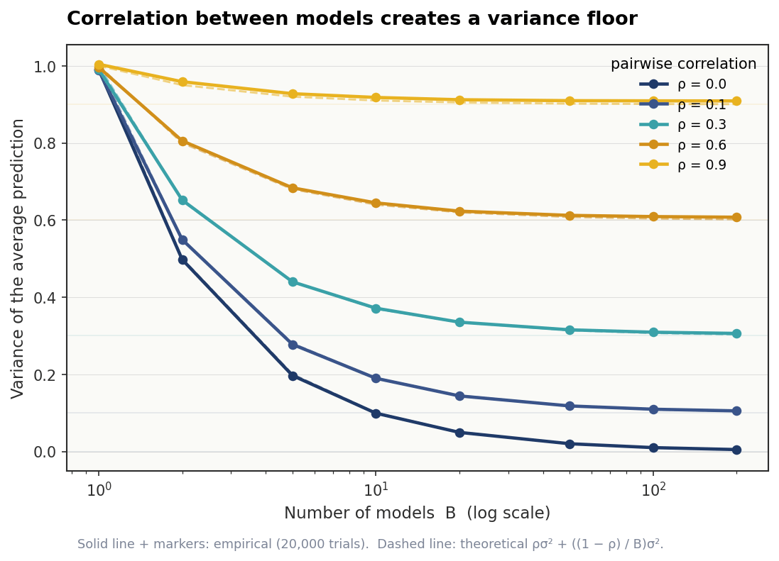
Two takeaways:
