Issue #132 - Bagging: Why Training on Broken Copies of Your Data Works

💊 Pill of the week

Bootstrap Aggregating is one of the cleanest ideas in machine learning. Here’s a full treatment: where it came from, why it works, what its limits are, and what it quietly gets wrong.

In this issue we will cover the following:

• What bagging is and why it works

• The free validation it gives you (OOB) and how many trees you actually need

• What it can’t fix: bias and correlated trees

• A notebook with all the code at the end!💎

🗓️And this Wednesday an extra issue only for paid subs💎

covering 7 related experiments

Interested in sponsoring MLPills?

• Contact me here:

• Or send me an email: mlpills23@gmail.com

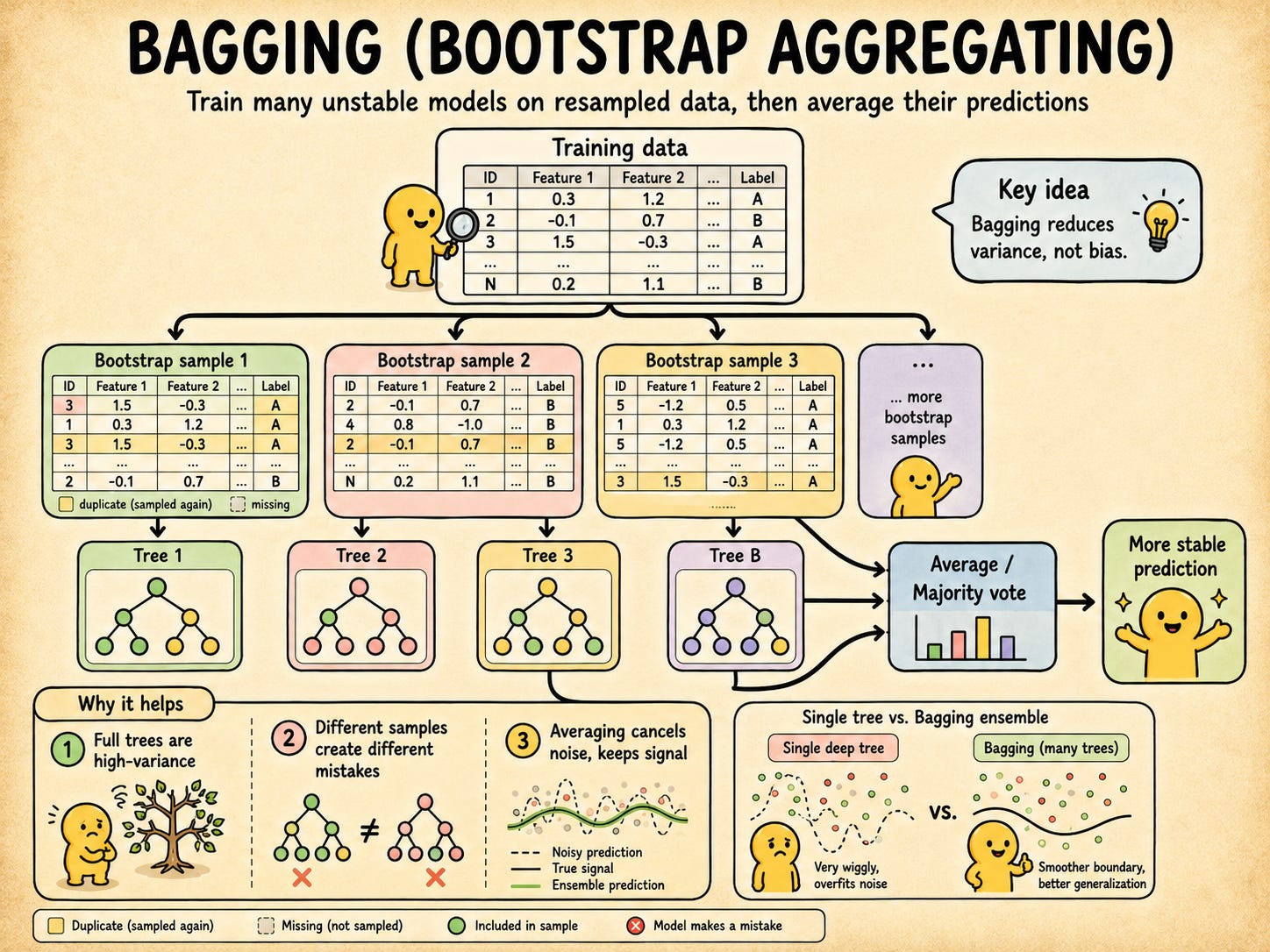
Leo Breiman published “Bagging Predictors” in 1996. The paper is short. The idea is even shorter: train many copies of the same model on slightly different versions of your data, then average their predictions.

That’s genuinely all it is.

What makes it worth unpacking is why it works, because the reasoning isn’t obvious at first glance, and once you see it, you immediately understand what bagging can’t do either.

The thing decision trees get wrong

A decision tree trained to full depth will memorize your training data. Not approximately. Actually memorize it. Change a handful of rows in the training set and you can get a completely different tree structure with different splits, different depth, different predictions.

This is the core problem. The model is chasing noise, not signal. So when you ask it to predict on data it’s never seen, it has no idea what it’s doing.

Model Variance How much a model’s predictions shift when trained on different samples of the same data. High variance means the model is very sensitive to which specific rows it trained on. Low variance means it would produce similar predictions regardless.

Overfitting and high variance are really the same problem described differently. Overfitting is what it does to your training data. Variance is how it behaves across different training sets.

Bagging attacks variance directly.

What “bootstrap” actually means?

The first word in Bootstrap Aggregating comes from Efron’s 1979 resampling technique. The idea was originally about estimating uncertainty in statistics, but Breiman borrowed it.

Given a training set of n rows: sample n rows from it, with replacement. Some rows show up twice. Some show up three times. Some never show up at all. The resulting dataset is the same size as your original, just shuffled and duplicated in a new way.

Bootstrap Sample A dataset created by drawing n times from an n-row training set, with replacement. Any row can appear zero, one, or multiple times. Each bootstrap sample is the same size as the original but contains a different mix of rows.

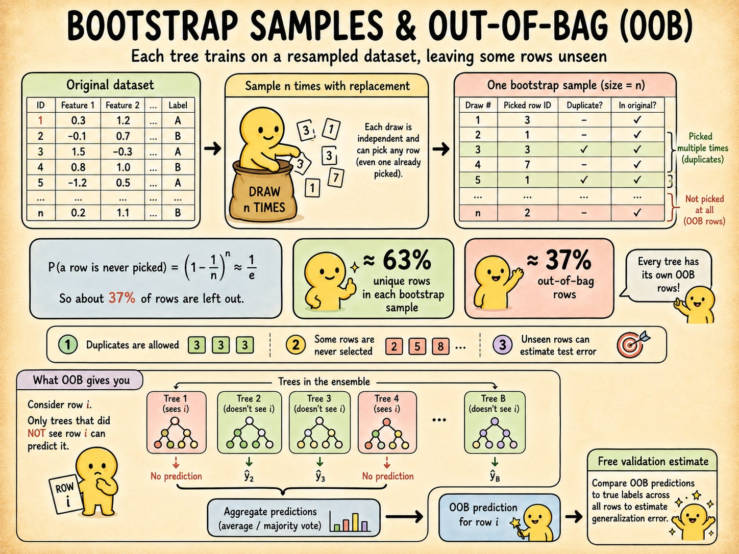
A natural question: how many unique rows survive? Each row has a 1/n chance of being picked on any single draw, so the probability of a specific row being skipped across all n draws is:

\(P(\text{row excluded}) = \left(1 - \frac{1}{n}\right)^n\)

For large n, this converges to 1/e, roughly 0.368. So about 63% of your original rows end up in any bootstrap sample. The other 37% were never selected.

You can confirm this in a few seconds with this code:

import numpy as np

rng = np.random.default_rng(42)
n = 1000

unique_fractions = []
for _ in range(500):
    sample = rng.integers(0, n, size=n)  # draw n indices with replacement
    unique_fractions.append(len(np.unique(sample)) / n)

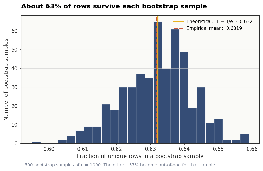
print(f"Mean unique fraction: {np.mean(unique_fractions):.4f}")

Mean unique fraction: 0.6319

This lines up almost exactly with the theoretical 1 - 1/e ≈ 0.6321 derived earlier. Roughly 63% of the original rows make it into any given bootstrap sample, and the remaining 37% become out-of-bag.

A helper function that returns both the sample and the out-of-bag mask:

def bootstrap_sample(X, y, rng):
    n = len(X)
    indices = rng.integers(0, n, size=n)
    oob_mask = np.ones(n, dtype=bool)
    oob_mask[indices] = False        # rows that were never drawn
    return X[indices], y[indices], oob_mask

Why averaging fixes anything

Train B models on B bootstrap samples. Average their predictions for regression, or take a majority vote for classification.

\(\hat{y}_{\text{bag}}(x) = \frac{1}{B} \sum_{b=1}^{B} \hat{y}_b(x)\)

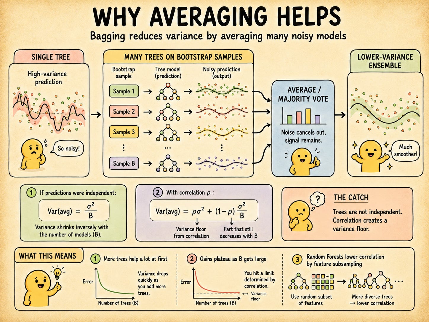
Why does this help? Basic probability: if you average B independent random variables each with variance σ², the average has variance σ²/B. More models means lower variance. The noise washes out, the shared signal survives.

Variance of an Average For B independent predictions each with variance σ², their average has variance σ²/B. This only holds if the predictions are independent. Correlation between models weakens this reduction.

And here’s the catch: bagged models are not independent. They all came from the same original dataset using the same algorithm. Their predictions will correlate, and that correlation sets a hard floor on how much averaging can help.

When predictions have pairwise correlation ρ, variance doesn’t go to zero:

\(\text{Var}(\hat{y}_{\text{bag}}) = \rho\sigma^2 + \frac{1-\rho}{B}\sigma^2\)

As B gets large, the right term disappears. What’s left is ρσ². Adding more trees can’t move this floor. Only reducing correlation between trees can.

This is the most useful thing to understand about bagging. It explains why Random Forests exist (feature subsampling lowers ρ) and why adding 500 trees instead of 200 rarely changes much.

Building this from scratch makes the loop obvious:

from sklearn.tree import DecisionTreeClassifier

class BaggingClassifierFromScratch:
    def __init__(self, n_estimators=100, random_state=0):
        self.n_estimators = n_estimators
        self.rng = np.random.default_rng(random_state)
        self.trees = []
        self.oob_indices = []

    def fit(self, X, y):
        n = len(X)
        for _ in range(self.n_estimators):
            X_boot, y_boot, oob_mask = bootstrap_sample(X, y, self.rng)
            tree = DecisionTreeClassifier()
            tree.fit(X_boot, y_boot)
            self.trees.append(tree)
            self.oob_indices.append(np.where(oob_mask)[0])
        return self

    def predict_proba(self, X):
        probs = np.mean([t.predict_proba(X) for t in self.trees], axis=0)
        return probs

    def predict(self, X):
        return np.argmax(self.predict_proba(X), axis=1)

    def oob_score(self, X, y):
        n = len(X)
        oob_preds = np.zeros((n, len(np.unique(y))))
        oob_counts = np.zeros(n)
        for tree, oob_idx in zip(self.trees, self.oob_indices):
            if len(oob_idx) == 0:
                continue
            oob_preds[oob_idx] += tree.predict_proba(X[oob_idx])
            oob_counts[oob_idx] += 1
        valid = oob_counts > 0
        preds = np.argmax(oob_preds[valid], axis=1)
        return np.mean(preds == y[valid])

The full algorithm is that loop. Everything else is bookkeeping.

You get a free validation score

Remember the ~37% of rows that never made it into a given tree’s training data? Those rows are genuinely unseen by that tree. That makes them a valid test set.

For each row in your training data, collect predictions only from trees that were trained without it, then compare to the true label. That’s the out-of-bag error estimate.

Out-of-Bag (OOB) Error A performance estimate computed by predicting each training row using only trees that didn’t include that row in their bootstrap sample. Because those trees never saw the row during training, the estimate approximates test error without needing a separate validation set.

sklearn makes this one parameter:

from sklearn.ensemble import BaggingClassifier
from sklearn.tree import DecisionTreeClassifier
from sklearn.datasets import make_classification
from sklearn.model_selection import train_test_split

X, y = make_classification(n_samples=1000, n_features=20, random_state=42)
X_train, X_test, y_train, y_test = train_test_split(X, y, test_size=0.2, random_state=42)

bag = BaggingClassifier(
    estimator=DecisionTreeClassifier(),
    n_estimators=200,
    oob_score=True,
    random_state=42,
    n_jobs=-1
)
bag.fit(X_train, y_train)

print(f"OOB accuracy:  {bag.oob_score_:.4f}")
print(f"Test accuracy: {bag.score(X_test, y_test):.4f}")

OOB accuracy:  0.9137
Test accuracy: 0.9000

The two scores land within about 1.4 points of each other, which is exactly the behavior we'd want from a free validation estimate. OOB ran a touch optimistic here, but not enough to be misleading. On a different seed or dataset the gap can flip the other way; what matters is that the magnitudes track.

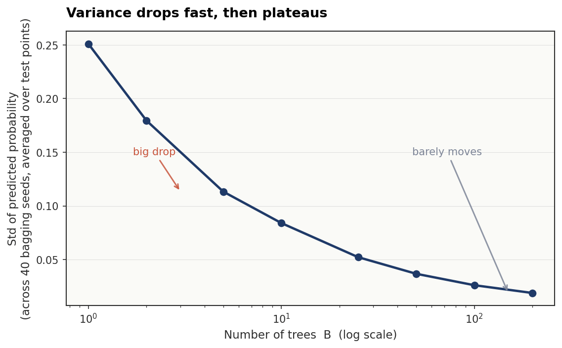
How many trees do you actually need?

Variance drops fast at first, then barely moves. Going from 1 tree to 10 makes a real difference. Going from 100 to 200 trees usually doesn’t.

OOB error stabilizes around B = 100 to 200 for most tabular datasets. Past that, you’re mostly spending compute. One useful property: unlike single trees, bagged ensembles don’t overfit as you add more trees. A deeper tree overfits. More trees don’t. These are separate knobs.

X, y = make_classification(n_samples=500, n_features=20, random_state=0)

single_scores, bagged_scores = [], []

for seed in range(50):
    X_tr, X_te, y_tr, y_te = train_test_split(X, y, test_size=0.3, random_state=seed)

    single = DecisionTreeClassifier().fit(X_tr, y_tr)
    bagged = BaggingClassifier(n_estimators=100, random_state=seed, n_jobs=-1).fit(X_tr, y_tr)

    single_scores.append(single.score(X_te, y_te))
    bagged_scores.append(bagged.score(X_te, y_te))

print(f"Single tree  | mean: {np.mean(single_scores):.3f}, std: {np.std(single_scores):.3f}")
print(f"Bagged (100) | mean: {np.mean(bagged_scores):.3f}, std: {np.std(bagged_scores):.3f}")

Single tree  | mean: 0.848, std: 0.034
Bagged (100) | mean: 0.884, std: 0.028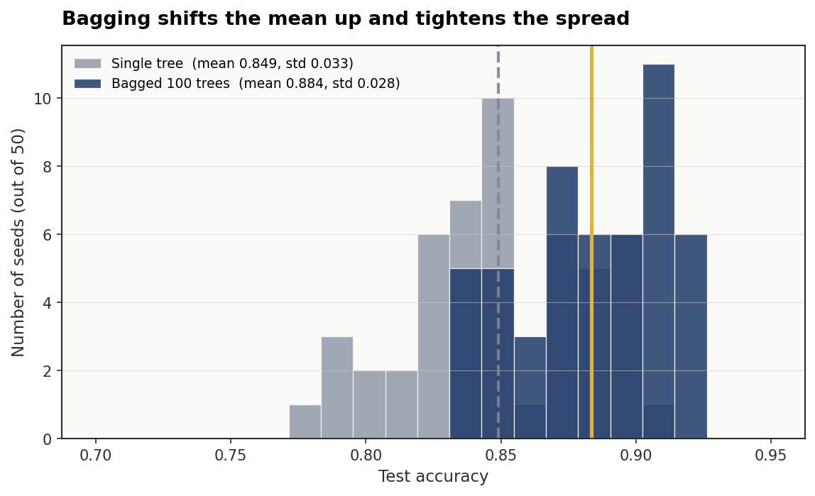

The mean accuracy climbs by roughly 3.6 points and the standard deviation across seeds tightens from 0.034 to 0.028. The worst single-tree runs get pulled up while the best ones barely move, which is exactly the signature of variance reduction. The ensemble isn't doing anything cleverer than a single tree on any given split, it's just refusing to be unlucky.

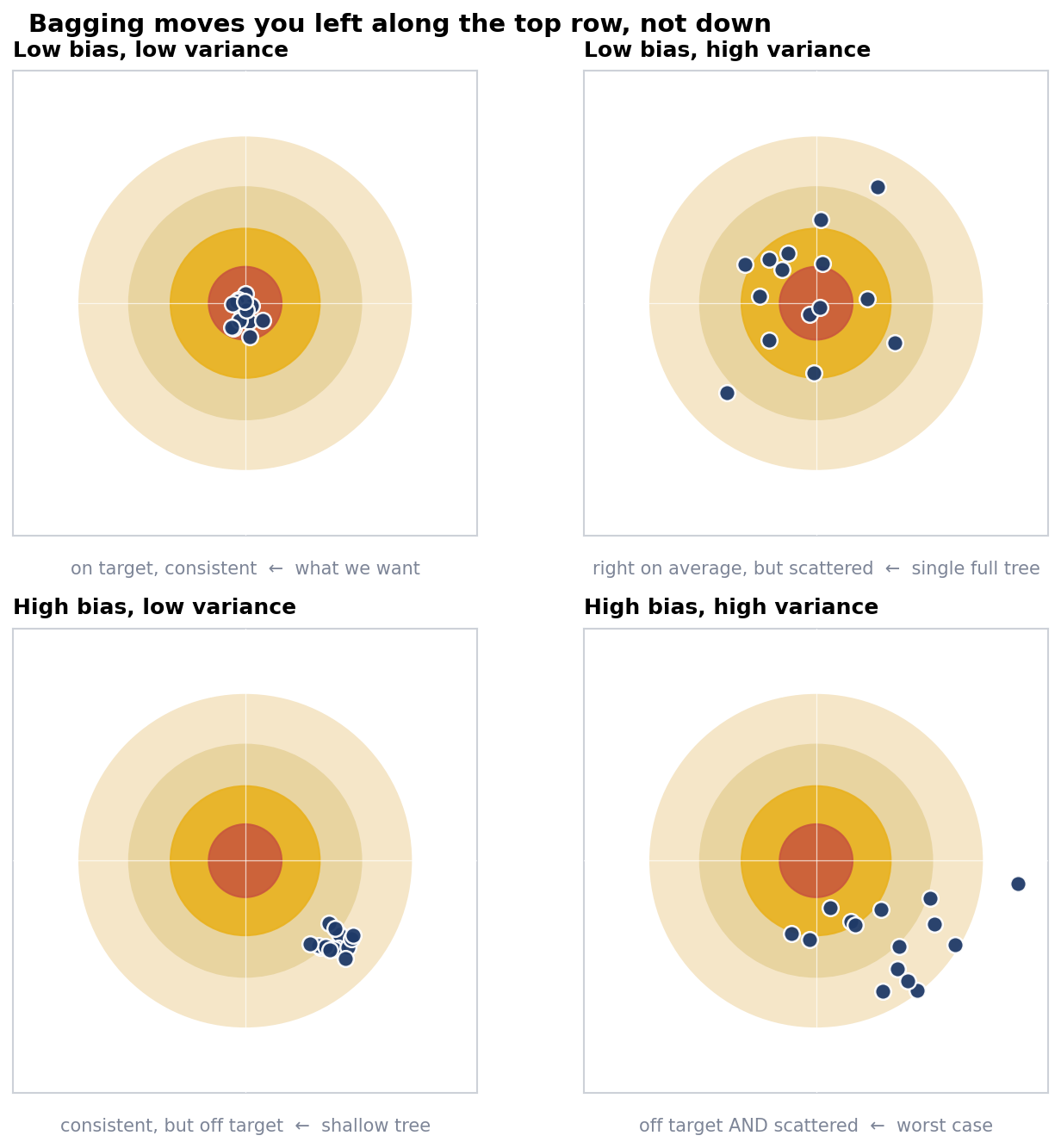
What bagging can’t fix

Bagging only fixes variance.

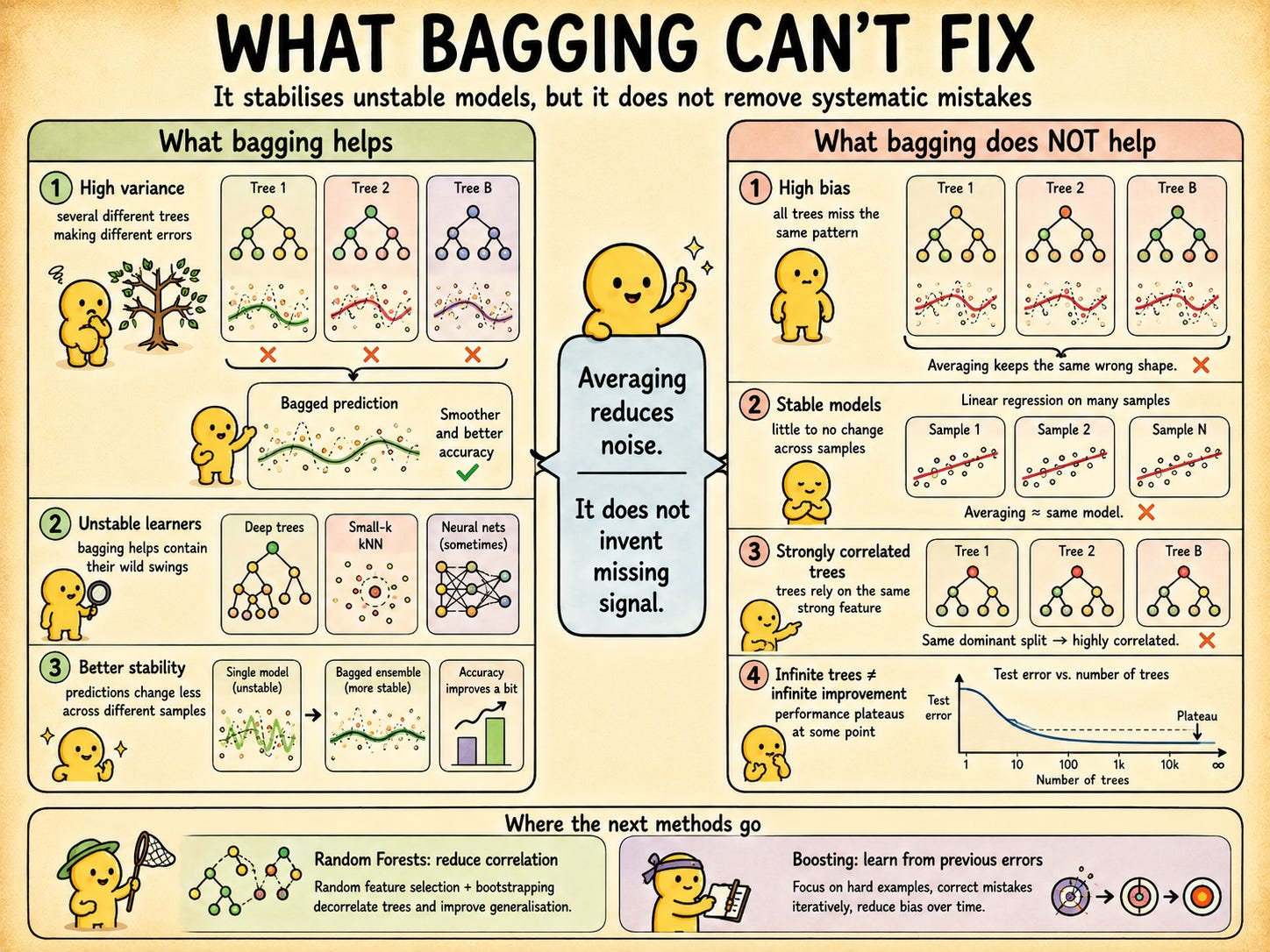
If your individual trees are all systematically wrong in the same direction, averaging them produces a prediction that’s still systematically wrong, just with less noise around it.

Model Bias The systematic error in a model’s predictions, regardless of the training sample. A high-bias model makes the same kinds of mistakes no matter what data it sees. Bias doesn’t cancel when you average predictions.

Say the true relationship in your data involves a feature interaction that no single tree reliably captures. Every tree misses it in roughly the same way. The average misses it too. Bagging on a bad model gives you a more stable bad model.

Correlated trees are the other thing bagging can’t fix. When one feature dominates the dataset, it shows up near the root of almost every tree regardless of which bootstrap sample that tree saw. Their predictions correlate, ρ stays high, and the variance floor doesn’t move. This exact failure mode is why Random Forests add feature subsampling at each split.

It works on more than trees

Bagging works on any high-variance model. The base learner doesn’t need to be a tree.

k-nearest neighbors with small k changes dramatically with small changes in training data, so it bags well. Neural networks are high-variance and benefit from ensemble averaging, though training 100 networks is rarely practical. Linear regression is inherently stable, so bagging it does almost nothing.

The prerequisite is instability. A model that’s already stable will produce correlated predictions on every bootstrap sample, and you’re back to ρ near 1.

Feature importance as a side effect