Issue #107 - Gaussian Mixture Models

💊 Pill of the week

Today we will introduce Gaussian Mixture Models (GMMs)! While K-Means is a fantastic starting point for clustering, it makes a rigid assumption: that clusters are spherical. GMMs relax this assumption, viewing clusters as originating from different Gaussian (normal) distributions. This allows for more flexible, elliptically shaped clusters and provides a probabilistic perspective on where each data point belongs.

At its core, a GMM is a probabilistic model that assumes all the data points are generated from a mixture of a finite number of Gaussian distributions with unknown parameters. Instead of assigning a point to a single cluster (hard assignment), GMMs provide a probability of that point belonging to each of the clusters (soft assignment). This nuanced approach makes GMMs a powerful tool for modeling complex data structures that K-Means might misinterpret.

You can review K-Means before moving to this week’s article:

Issue #106 - Introduction to K-means clustering

How does it work?

The magic behind GMMs is the Expectation-Maximization (E-M) algorithm. It's an iterative process that finds the maximum likelihood parameters of the underlying Gaussian distributions. Think of it as a two-step dance the algorithm performs until it finds the best possible fit for the data.

The working mechanism of E-M for GMMs can be described as follows:

1. Initialization: The algorithm begins by initializing K Gaussian distributions. This involves setting initial values for the mean (μ_k), covariance (Σ_k), and mixing coefficient (π_k) for each cluster k. A common strategy is to first run K-Means to find initial cluster centers.

2. Expectation Step (E-step): In this step, the algorithm calculates the probability (or "responsibility") of each data point x_i belonging to each cluster k. This is a soft assignment, where for every point, we get a set of probabilities that sum to 1. The responsibility r_ik is calculated using the current parameters of the Gaussians.

   \(r_{ik} = \frac{\pi_k \mathcal{N}(x_i | \mu_k, \Sigma_k)}{\sum_{j=1}^{K} \pi_j \mathcal{N}(x_j | \mu_j, \Sigma_j)}\)

3. Maximization Step (M-step): Using the responsibilities from the E-step, the algorithm updates the parameters for each Gaussian to maximize the likelihood of the data. Essentially, it refits the Gaussians to the data, with each data point's influence weighted by its responsibility.

4. Iteration & Convergence: The E-step and M-step are repeated iteratively. With each cycle, the algorithm refines the parameters, getting closer to a solution that best explains the data. The algorithm converges when the change in the total log-likelihood of the data between iterations falls below a certain threshold.

GMM in action

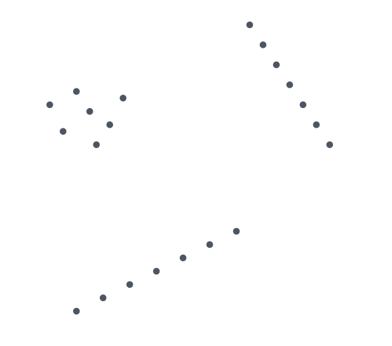
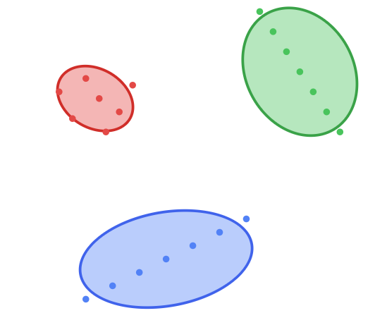
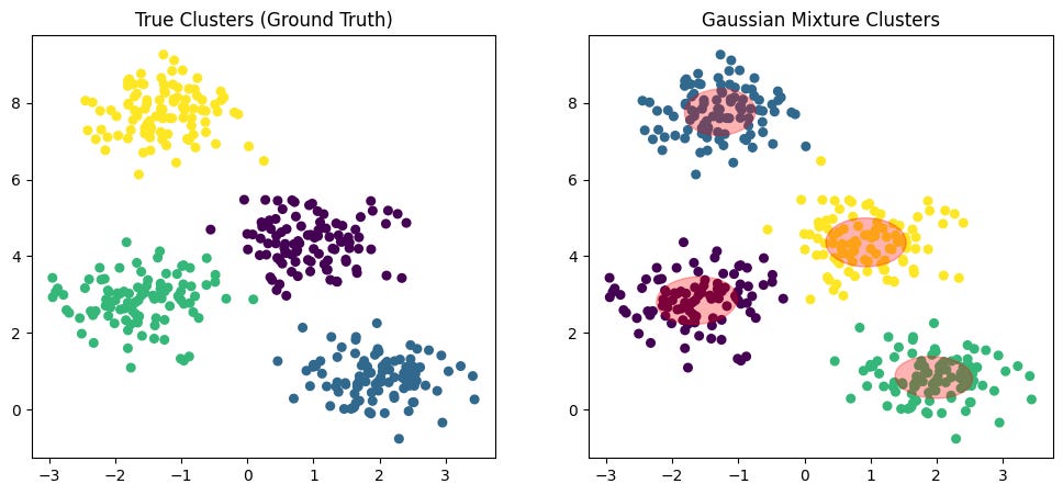
Let's see it in action with an example. This is our initial data. We can see that we have 3 clusters, and they are elliptical, not spherical. The algorithm doesn't know the cluster assignments yet; all points are treated as part of one dataset.

Initialization: To make the example simple, let's select K equal to 3. We initialize 3 Gaussian distributions. Notice they start as simple circles, representing our initial "guess" for the clusters' positions and shapes. They have no knowledge of the underlying data structure yet.

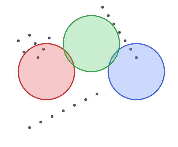
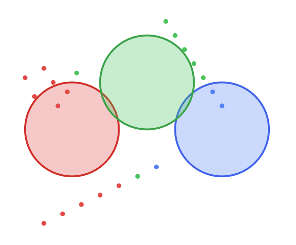
Expectation Step (E-step): Now, the E-Step happens. Each data point is softly assigned a probability of belonging to each of the three initial Gaussians. The colors of the data points now represent the most likely cluster for each point, based on its proximity to the initial circles.

Maximization Step (M-step): Next, the M-Step. The parameters of the Gaussians (mean, covariance) are updated based on these probabilistic assignments. The circles stretch and rotate into ellipses to better fit the data points now assigned to them. You can see them moving and reshaping to better capture their respective clusters.

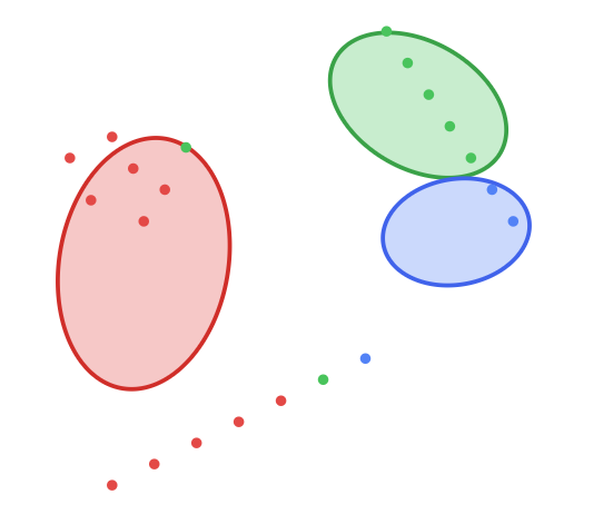
Iteration & Convergence: We check for convergence by seeing if the assignments and Gaussian parameters have stabilized. After repeating the E-Step and M-Step a few more times, the process ends. We get a perfect fit, with each ellipse accurately describing the location, shape, and orientation of its respective cluster.

When to Use it?

Gaussian Mixture Models are particularly well-suited for the following scenarios:

• Clustering Non-Spherical Data: When your clusters are elongated or have different orientations (elliptical), GMMs will outperform K-Means.

• Density Estimation: GMMs can model the underlying probability distribution of the data, which is useful for understanding how your data is structured.

• Anomaly Detection: Points that have a very low probability of belonging to any of the Gaussian components can be flagged as outliers.

• Image Segmentation: GMMs can cluster pixels based on color, providing soft assignments that can lead to more natural segmentation boundaries.

• Generative Modeling: Since a GMM learns the data's distribution, you can use it to generate new synthetic data points that resemble the original data.

Pros and Cons

Pros:

• Flexible Cluster Shapes: Does not assume clusters are spherical and can model elliptical shapes.

• Soft Clustering: Provides probabilistic assignments, offering more nuance than the hard assignments of K-Means.

• Statistically Grounded: Based on the well-defined statistical theory of maximum likelihood estimation.

• Provides Density Estimation: Not just a clustering algorithm, but also a model of the data's probability distribution.

Cons:

• Computationally Intensive: The E-M algorithm is more complex and slower than the K-Means algorithm.

• Requires Specifying K: Like K-Means, you must choose the number of components in advance.

• Sensitive to Initialization: A poor start can lead to slow convergence or a suboptimal solution.

• Complexity: Can be prone to overfitting if the number of components is too high for the amount of data available.

Python Implementation

Here's a basic example of using GMMs with the scikit-learn library:

from sklearn.mixture import GaussianMixture

# Fit a Gaussian Mixture Model (GMM)
gmm = GaussianMixture(n_components=3, random_state=42)
gmm.fit(X)  # X = your data

# Hard cluster assignments
labels = gmm.predict(X)

# Soft cluster assignments (probabilities)
probs = gmm.predict_proba(X)

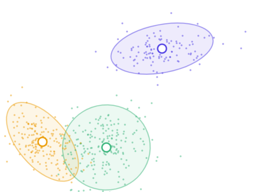
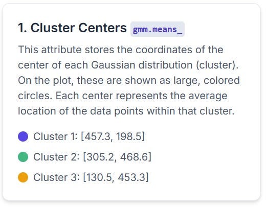
Interpreting the Results

The key outputs from a GMM that can be interpreted are:

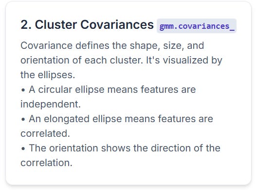
• Means (model.means_): The coordinates of the center of each Gaussian component.

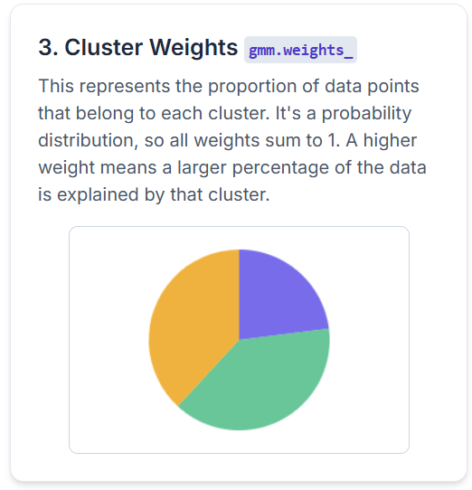
• Covariances (model.covariances_): A matrix for each component describing its shape and orientation.

• Weights (model.weights_): The mixing coefficients, representing the proportion of the data belonging to each cluster.

• Log-Likelihood: The log of the probability of the data given the model. It's used to assess model fit (higher is better).

You can extract and analyze these outputs like this:

# Cluster centers
cluster_centers = gmm.means_

# Cluster covariances (shape and orientation)
cluster_covariances = gmm.covariances_

# Cluster weights (proportion of data)
cluster_weights = gmm.weights_

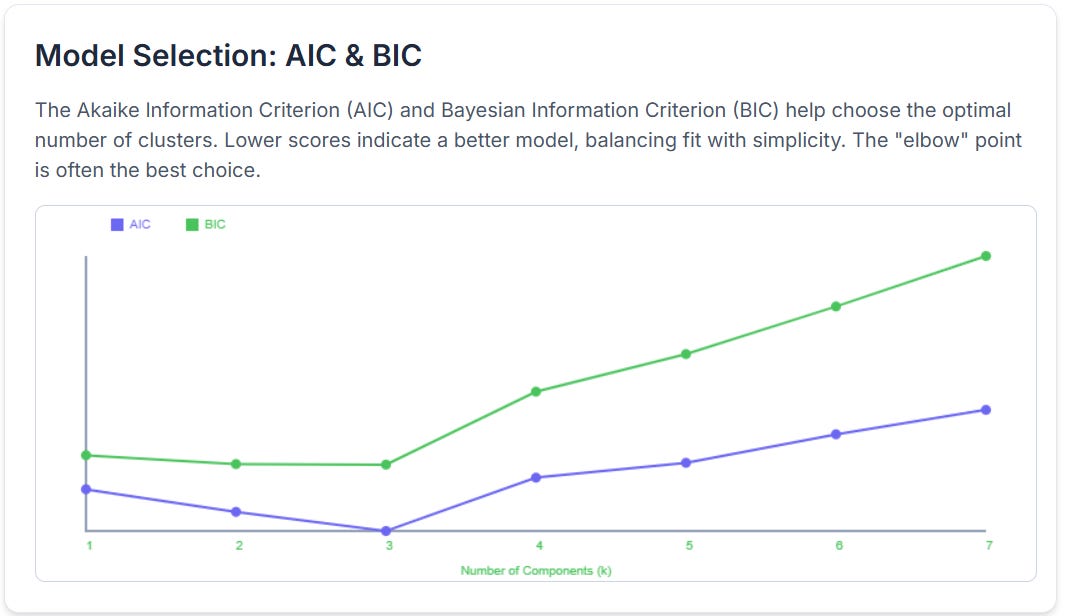
# AIC and BIC for model selection
aic_score = gmm.aic(X)
bic_score = gmm.bic(X)

Let’s see each component in practice. Let’s imagine this data:

Conclusion

Gaussian Mixture Models offer a powerful and flexible alternative to K-Means. By embracing a probabilistic approach and modeling clusters as Gaussian distributions, GMMs can capture complex, non-spherical structures that other algorithms miss. While they are more computationally demanding, their ability to provide soft assignments and a generative model of the data makes them an invaluable tool for density estimation, anomaly detection, and sophisticated clustering tasks.

---

⚡️Power-Up Corner

Now that you’ve seen how GMMs work, let’s explore the advanced features that make them so versatile.

Choosing the Optimal Number of Clusters with AIC and BIC

With K-Means, we use the "Elbow Method." For GMMs, we have more statistically robust tools: the Akaike Information Criterion (AIC) and the Bayesian Information Criterion (BIC).