


💊 Pill of the Week
In Part 1, we set up the problem: causal effects are defined by counterfactuals, and counterfactuals are never observed. In Part 2, we worked through the classical estimation toolkit, from randomised experiments to adjustment methods and quasi-experimental designs.


Those methods mostly answer one question: what is the average effect? That is often enough for a go or no-go decision, but averages hide the structure that matters most in practice.
A drug with zero average effect might save one subgroup and harm another. A retention campaign with a modest average lift might be brilliant for 20% of customers and actively counterproductive for another 20%. If you only ever look at the average, both systems look boring, and you keep spending money in the wrong places.
This final part is about the ML side of causal inference: estimating how effects vary across people, then turning those estimates into targeting decisions.
In this series
Part 1: foundations, frameworks, and the fundamental problem
Part 2: RCTs, adjustment-based methods, and quasi-experimental designs
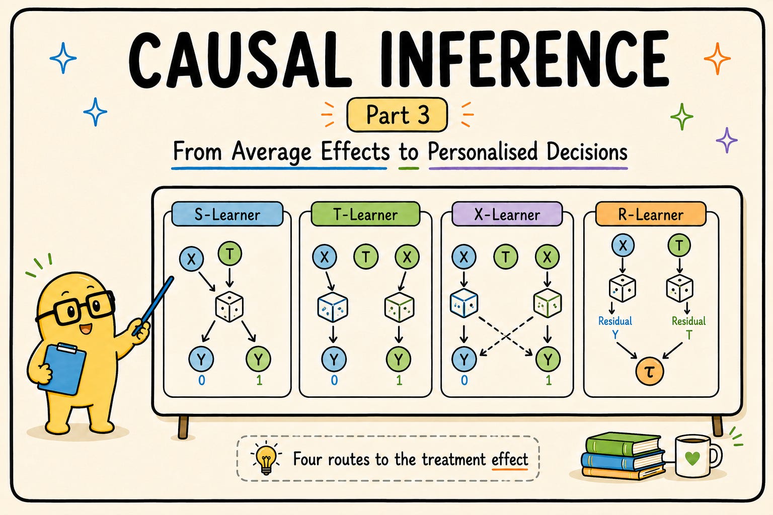
Part 3: meta-learners, Double Machine Learning, causal forests, uplift modelling, causal discovery, and the tooling ecosystem
The target: CATE
Recall the Conditional Average Treatment Effect from Part 1:
In words, this is the expected treatment effect for units whose features look like x. It sits behind every personalisation question:
Medicine: which patients benefit from this therapy, and for whom is it neutral or harmful?
Marketing: which prospects does this campaign actually persuade?
Retention: whose churn does this offer prevent?
Education: which students benefit most from tutoring, so a limited budget goes furthest?
Public policy: which households does a job-training programme help?
But remember the catch: the individual effect Y(1)-Y(0) is never observed for anyone. We see the treated outcome or the untreated outcome, never both.
The fundamental problem of causal inference:
only one potential outcome is observable.
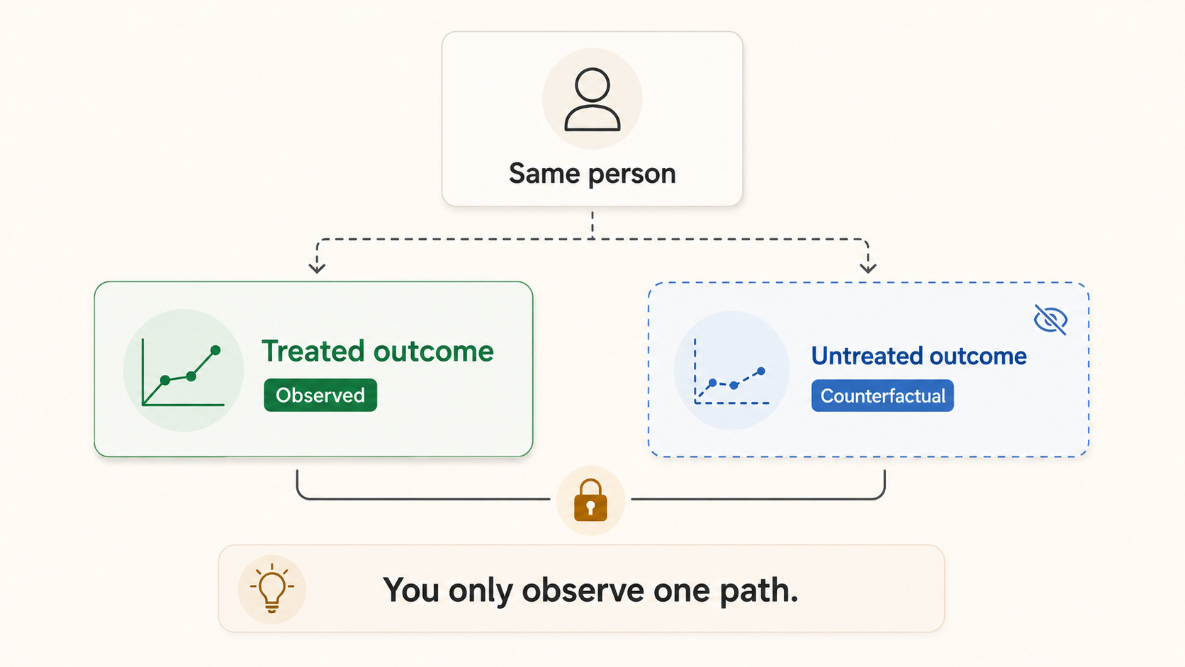
So CATE estimation is supervised learning where the label does not exist. You never fit a model directly to the quantity you care about. Instead, you fit models to observable outcomes and then difference, residualise, or split your way towards the effect.
Meta-learners
Meta-learners wrap ordinary supervised models, whether XGBoost, LightGBM, a neural network, or whatever you already run in production, into CATE estimators.
They work best with experimental data. They can also extend to observational data under the unconfoundedness assumption, with propensity adjustments doing much of the work.
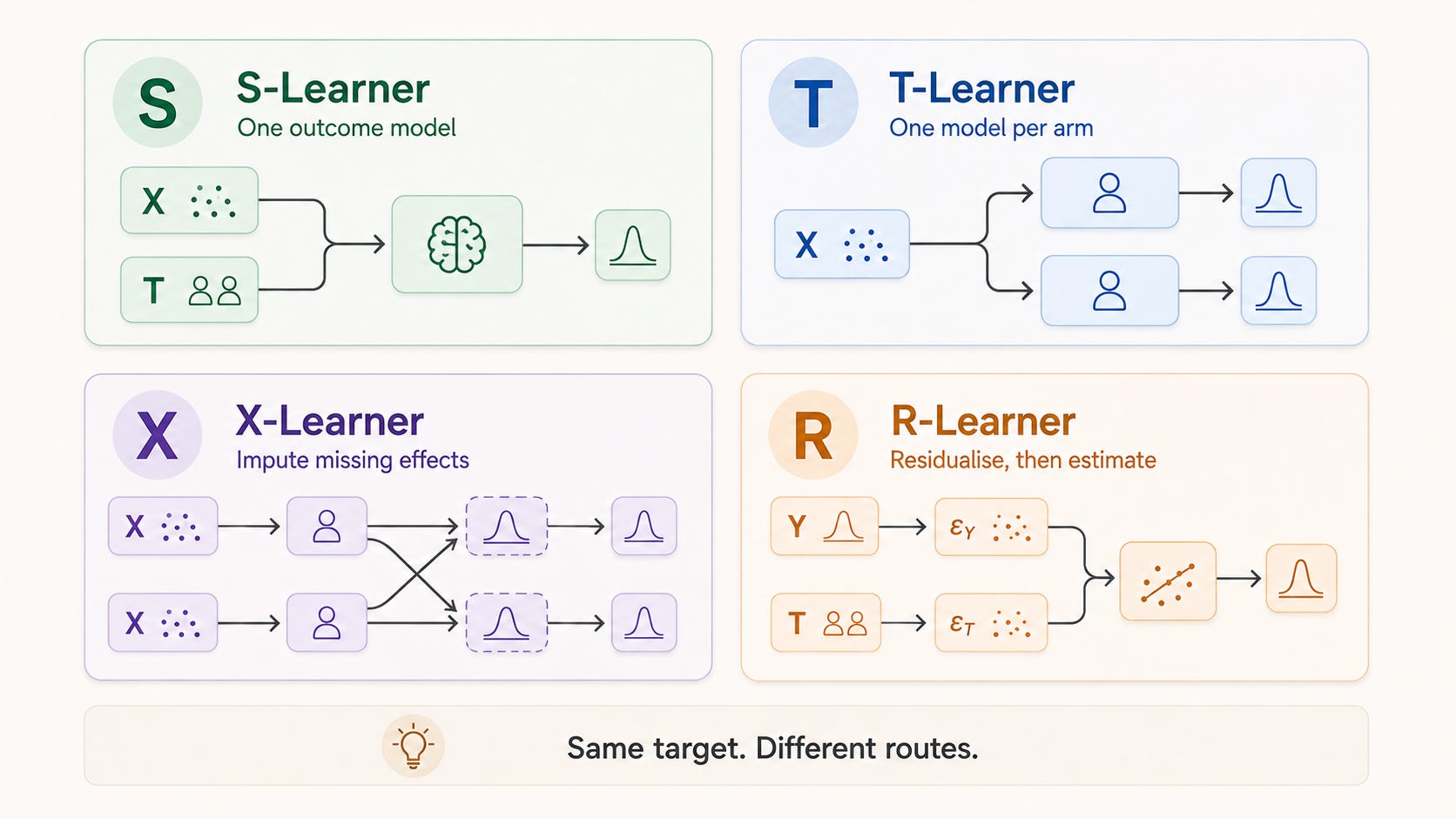
The four core approaches differ mainly in how they divide the data and where they allow bias to enter.
The S-Learner is the simplest, most data-efficient baseline: one outcome model receives treatment as a feature. Its main risk is that regularisation can suppress small treatment effects.
The T-Learner fits a separate outcome model for each treatment arm. This flexibility helps when the response surfaces genuinely differ, but treatment imbalance and uneven smoothing can create misleading differences.
The X-Learner builds on those two models by imputing missing effects and combining the resulting estimates. It is especially useful when one treatment arm is much smaller, although it introduces more nuisance models and moving parts.
The R-Learner, closely related to Double Machine Learning, residualises both treatment and outcome before estimating the effect. It is the strongest choice when inference and confidence intervals matter, provided cross-fitting is implemented carefully.
1. S-Learner
Train a single model f(X,T) with treatment as another feature, then compare its two predictions:
It is simple and data-efficient, with only one model to maintain and monitor.
The weakness is regularisation. If the treatment effect is small relative to the baseline signal, as it usually is, the model has little incentive to use the treatment feature. It shrinks towards zero, and the estimated effects shrink with it.
An S-Learner that reports no heterogeneity is not evidence that no heterogeneity exists.
2. T-Learner
Train one model per arm, f₁ on treated units and f₀ on controls, then take the difference:
Each model can capture arm-specific structure, which is exactly what you want when the treated and untreated response surfaces genuinely differ.
The weakness is that each model only sees part of the data. Any difference in how the models are regularised can masquerade as a treatment effect. If f₁ is fitted on 5,000 rows and f₀ on 500,000, they will not smooth in the same way. Their difference contains that artefact alongside the real signal.
3. X-Learner
The X-Learner is designed for treatment-control imbalance. Its central idea is to impute the missing half of the story.
First, fit the two T-Learner outcome models. For each treated unit, subtract f₀’s prediction of its untreated outcome from its observed outcome. For each control unit, take the mirror image. These become imputed individual effects.
Next, fit models to those imputed effects and combine their estimates using the propensity score, leaning on whichever arm has more support in that region of feature space.
When you have 5% treated and 95% control, a common industry holdout design, this can extract considerably more information from the smaller arm than a plain T-Learner.
4. R-Learner and Double Machine Learning
This is the most statistically principled member of the family. The core idea is Robinson residualisation, revived and generalised through Double Machine Learning:
Predict the outcome from the covariates, m(X) = E[Y | X], then compute Y − m(X).
Predict treatment from the covariates, e(X) = E[T | X], then compute T − e(X).
Regress the outcome residuals on the treatment residuals to estimate the effect.
You remove everything the covariates can explain about both the outcome and treatment assignment. Then you ask whether what remains of treatment still moves what remains of the outcome.
Two properties make this more than a neat trick:
Cross-fitting trains the nuisance models on one fold and computes residuals on another, reducing overfitting bias.
Neyman orthogonality makes the causal estimate less sensitive to small nuisance-model errors, enabling valid confidence intervals.
This is the method to reach for when a stakeholder asks the reasonable follow-up question: yes, but what is the error bar?
Causal forests
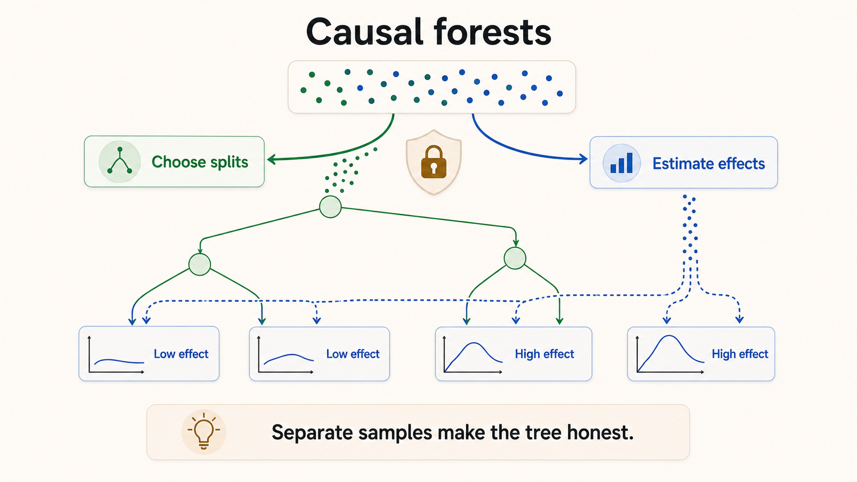
Wager and Athey’s causal forests adapt random forests to estimate CATE directly, rather than by differencing two predictions. Two modifications make them causal.
First, splits are selected to maximise treatment-effect heterogeneity between child nodes, not to reduce ordinary prediction error. The tree looks for places where the effect changes, not simply where the outcome changes.
Second comes honesty. Within each tree, one subsample chooses the splits and a disjoint subsample estimates effects inside the leaves. That separation supports asymptotically valid confidence intervals at the individual level, which is rare and genuinely useful.
Causal forests are a strong default for tabular CATE problems: non-parametric, reasonably robust, and equipped with uncertainty estimates. The grf package in R and EconML’s CausalForestDML in Python are the standard implementations.
Uplift modelling: CATE in production
Uplift modelling is the industry-facing version of CATE estimation. It dominates CRM, retention, telecoms, insurance, banking, and promotional targeting because it asks the operational question directly: who changes behaviour because of the intervention?
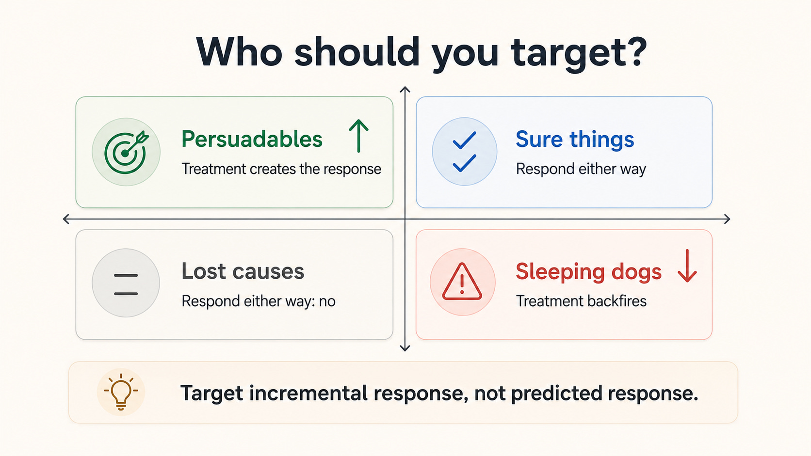
The framing divides an audience into four groups:
Persuadables respond only if treated. These are the people worth spending on.
Sure things respond either way. Treating them burns budget, or margin when the treatment is a discount.
Lost causes respond neither way. Treatment is also wasted here.
Sleeping dogs respond negatively to treatment. Think of a renewal reminder that prompts cancellation or a win-back email that triggers an unsubscribe.
Here is the distinction worth internalising:
A response model ranks by P(respond). An uplift model ranks by the incremental change in that probability.
A conventional response model reliably concentrates spend on sure things because they are easiest to predict. An uplift model creates a different ordering, often a dramatically more profitable one.
How do you evaluate a model when the individual label is missing?
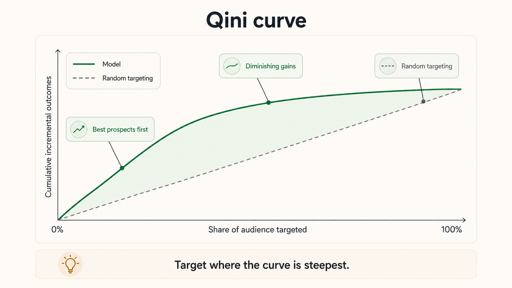
You need a randomised holdout and evaluation machinery designed for uplift. The standard tools are the Qini curve and Qini or uplift AUC.
Rank units by predicted uplift, sweep down the ranking, and plot cumulative incremental outcomes against the share of the population targeted. A good uplift model front-loads the gains, so its curve rises steeply and then flattens.
The useful targeting region is where the model curve rises fastest above random selection.
Two operational lessons
Protect the holdout. You need randomised data, or at least a permanent randomised control group, to train and honestly evaluate these models. That control group is the cost of doing business, and often the first thing someone tries to delete when targets are tight.
Expect drift. Effects change as populations, products, and channels evolve. Pairing a CATE model with an exploration layer, such as Thompson Sampling over targeting policies, helps prevent estimates from quietly going stale.
🔒 Paid-subscriber section
Become a 💎paid subscriber💎 to unlock
causal discovery
the tooling ecosystem
the practical workflow checklist
Final thoughts
Causal inference is not a replacement for predictive ML. It is the layer that turns predictions into decisions.
A readmission score tells a hospital who is at risk. A CATE model tells it which discharge intervention helps whom. A churn score tells you who might leave. An uplift model tells you who is worth saving, and what to send them.
Teams that internalise that distinction stop optimising proxy metrics and start optimising interventions. It is a slower and less comfortable way to work, but it is the one that compounds.
If there is appetite, the natural follow-up is a hands-on issue: build an uplift model with meta-learners on a public dataset, evaluate it with Qini curves, and watch it beat a naïve response model on the same data.
Reply and let me know if you want that issue next.
Happy learning!