

Issue #93 – Binning in Machine Learning

💊 Pill of the Week
Binning (also called discretization) is the process of transforming continuous numerical features into discrete categorical intervals, called bins.
It can help models by reducing noise, simplifying feature relationships, making linear models capture non-linearity, and improving interpretability.
However, binning also compresses information, so it should be applied carefully.
In this guide, we’ll explore 6 key binning methods, explain when and why to use each, their pros and cons, and how to interpret the binned features. Also accompanied with a code snippet so you can use it in your analysis.
💎All the code is shared at the end of the newsletter!💎
We will use the following made-up data:

That you can generate using this code:
import numpy as np
np.random.seed(42)
data = np.random.randn(100) * 15 + 50
X = data.reshape(-1, 1)
y = (data > 60).astype(int)
After binning your data you could check if these new features are relevant or not. Check this previous issue:

Let’s beging!
🥉Basic Binning Techniques
1. Equal-Width Binning
What it is:
Divides the range of a feature into N intervals of equal size (width), regardless of how the data is distributed.
When to use it:
Data is roughly uniformly distributed.
You want simple, equally spaced intervals for easy interpretation.
Quick exploratory data analysis (EDA) histograms.
Advantages:
Simple and intuitive.
Bins are easy to interpret (e.g., each bin spans 10 units).
Drawbacks:
Bins may be imbalanced (some bins could be empty if the data is skewed).
Not ideal for skewed or heavy-tailed distributions.
Interpretation:
Each bin represents a range with fixed width. A feature value belongs to a bin based on its raw magnitude, without regard to how many samples exist in that range.
Python Example:
import pandas as pd
import numpy as np

equal_width_bins = pd.cut(data, bins=4)
The outcome of this method is:
== Equal-Width Binning ==
(10.637, 27.474]     6
(27.474, 44.244]    32
(44.244, 61.014]    42
(61.014, 77.784]    20
Name: count, dtype: int64
This method created bins with fixed value ranges, but as expected with skewed data, the bin counts are uneven — most values fall into the middle two bins, while the lowest bin is sparsely populated. It’s simple, but less effective for non-uniform distributions.
2. Equal-Frequency (Quantile) Binning
What it is:
Divides the feature values into N bins, each containing (approximately) the same number of observations.
When to use it:
Data is skewed or unevenly distributed.
You want balanced bins with equal sample sizes.
Reducing the impact of outliers or long tails.
Advantages:
No empty bins.
Handles skewness and outliers naturally.
Useful for models sensitive to class imbalance across features.
Drawbacks:
Bin ranges can be uneven and unintuitive.
Small numeric differences could place samples into different bins.
Interpretation:
Each bin covers a different value range but holds a similar proportion of data points (e.g., 25% per quartile if q=4).
Python Example:
quantile_categories = pd.qcut(data, q=4)
print(pd.value_counts(quantile_categories).sort_index())
The outcome is:
== Equal-Frequency Binning ==
(10.703000000000001, 40.986]    25
(40.986, 48.096]                25
(48.096, 56.089]                25
(56.089, 77.784]                25
Name: count, dtype: int64
Each bin contains exactly 25 observations, showing how well this method balances bin sizes. The trade-off is that bin ranges are uneven, which can make interpretation less intuitive — but it’s ideal for handling skewed data and ensuring no empty bins.
While pd.qcut() aims to create bins with equal numbers of observations, exact equality isn't always guaranteed. If multiple values fall on a bin edge (quantile boundary), qcut may slightly adjust bin sizes to avoid splitting identical values across bins. As a result, some bins may contain one more or fewer values than expected. This is normal and helps preserve bin integrity in the presence of ties.
📖 Book of the week
If you're working with structured data — whether in finance, research, engineering, or tech — you need to check it out:
"Pandas Cookbook (3rd Edition)" By William Ayd & Matthew Harrison

This book isn’t just another cookbook — it’s a powerful, modern guide to solving real-world data problems with pandas 2.x. From quick fixes to scalable pipelines, it equips you with the tools to analyze, clean, merge, and visualize data with confidence and speed.
What sets it apart?
It helps you go from "getting things to work" to writing fast, clean, idiomatic pandas code like a pro:
✅ Master pandas' updated type system and core data structures
✅ Load, merge, reshape, group, and filter data with elegant, tested recipes
✅ Analyze time series and perform SQL-like operations on massive datasets
✅ Optimize memory usage and scale your analysis with PyArrow and databases
✅ Includes bonus content: code files, free PDF, and access to a private Discord
This is a must-read for:
🧠 Python developers
📊 Data analysts
🛠 Engineers dealing with high-volume or messy data
🔍 Data scientists aiming to master their data stack
If you want to take your pandas skills beyond the basics — and get faster, better, and more scalable at working with structured data — this book is for you.
🥈 Intermediate Binning Techniques
3. Custom Binning (Domain Knowledge)
What it is:
You manually define bin edges based on domain expertise, business rules, or external standards.
When to use it:
Clear domain thresholds exist (e.g., age groups, tax brackets).
Regulatory or operational rules must be reflected.
You want bins that are easy to explain to stakeholders.
Advantages:
Highly interpretable.
Aligns closely with real-world or business meanings.
Supports consistency across models and reports.
Drawbacks:
Risk of subjectivity or arbitrary cutoffs.
May not reflect the true statistical distribution of data.
Interpretation:
Each bin corresponds to a meaningful category (e.g., "Teen" = age 13–19). Easy to explain and act upon.
Python Example:
ages = pd.Series([5, 17, 18, 34, 45, 67, 89])
bins = [0, 12, 19, 64, np.inf]
labels = ["Child", "Teen", "Adult", "Senior"]
age_groups = pd.cut(ages, bins=bins, labels=labels)
print(age_groups)
The outcome is:
== K-Means Binning ==
Bin 0: Count = 17
Bin 1: Count = 34
Bin 2: Count = 29
Bin 3: Count = 20
Bin edges: [10.70382344 35.21363632 48.57673692 60.67263421 77.78417277]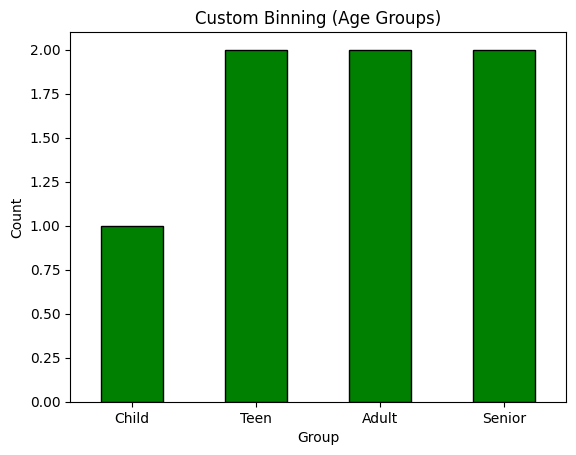
The binning clearly assigns each age to a human-understandable group (Child, Teen, Adult, Senior). This approach enhances interpretability and is useful when you have domain standards — but it doesn’t consider data distribution or model performance directly.
4. K-Means Binning (Clustering-Based)
What it is:
Uses the K-Means clustering algorithm to group values into N clusters along the value axis.
When to use it:
Data is multimodal or naturally forms groups.
You want bins that reflect natural separations rather than arbitrary cut points.
Advantages:
Adapts to the structure of the data.
Useful for irregular, non-uniform distributions.
Drawbacks:
Uneven sample sizes per bin.
Results can vary depending on initialization.
Requires choosing the number of bins carefully.
Interpretation:
Each bin captures a group of similar values found automatically by clustering. Boundaries may not be evenly spaced or easy to explain without visualization.
Python Example:
from sklearn.preprocessing import KBinsDiscretizer

X = data.reshape(-1, 1)
kbin = KBinsDiscretizer(n_bins=4, encode='ordinal', strategy='kmeans')
binned_kmeans = kbin.fit_transform(X)
print(kbin.bin_edges_[0])
The outcome is:
== Custom Binning (Age Groups) ==
   Age   Group
0    5   Child
1   17    Teen
2   18    Teen
3   34   Adult
4   45   Adult
5   67  Senior
6   89  Senior
This technique identified natural groupings in the data. The bin edges reflect the underlying structure of the distribution, and the bin sizes vary accordingly. It’s more adaptive than equal-width but less interpretable without visualization.
🎓Further Learning*
Are you ready to go from zero to building real-world machine learning projects?

Join the AI Learning Hub, a program that will take you through every step of AI mastery—from Python basics to deploying and scaling advanced AI systems.
Why Join?
✔ 10+ hours of content, from fundamentals to cutting-edge AI.
✔ Real-world projects to build your portfolio.
✔ Lifetime access to all current and future materials.
✔ A private community of learners and professionals.
✔ Direct feedback and mentorship.
What You’ll Learn:
Python, Pandas, and Data Visualization
Machine Learning & Deep Learning fundamentals
Model deployment with MLOps tools like Docker, Kubernetes, and MLflow
End-to-end projects to solve real-world problems
Take the leap into AI with the roadmap designed for continuous growth, hands-on learning, and a vibrant support system.
*Sponsored: by purchasing any of their courses you would also be supporting MLPills.
🥇Advanced Binning Techniques
5. Supervised / Optimal Binning (Target-Based)
Keep reading with a 7-day free trial
Subscribe to Machine Learning Pills to keep reading this post and get 7 days of free access to the full post archives.