


💎A Field Guide to Tree Models
As promised, here you have the companion notebook for the week’s article:

Here you have it:
Let’s see you what you’ll find in there:
The field guide told you how tree models differ. The companion notebook makes you prove it.
It builds one messy tabular problem and runs every family on it: a single CART tree, Random Forest, Extra Trees, AdaBoost, Gradient Boosting, Histogram Gradient Boosting, and Isolation Forest. Everything runs on numpy, pandas, matplotlib and scikit-learn. No extra installs.
The dataset is a simulated subscription conversion task. 12,000 rows, 5.99% positive rate, mixed numeric and categorical features, a nonlinearity, an interaction, missing values, and one useless high-cardinality ID column planted on purpose. Because the data-generating process is known, you can separate signal from artefact.
The notebook does not restate the article’s claims. It audits them.
Scaling really is irrelevant
Standardise the features. Log the income column. Refit the tree.
Maximum absolute prediction difference: 0 in both cases. Trees only use feature order, so any strictly monotonic transform preserves the candidate splits.
Extrapolation really is impossible
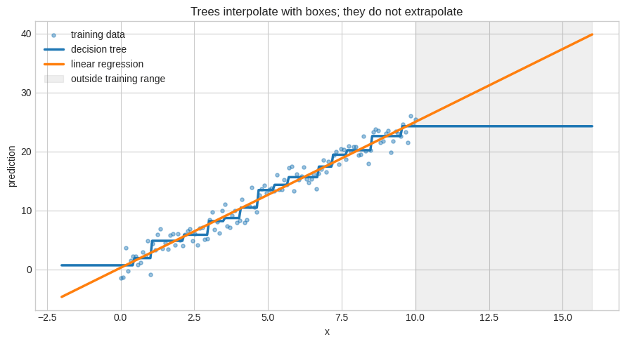
Past the training range the tree returns its terminal leaf forever. The linear fit keeps climbing. This is structural, and forests and boosted regressors inherit it.
No single metric ranks the models
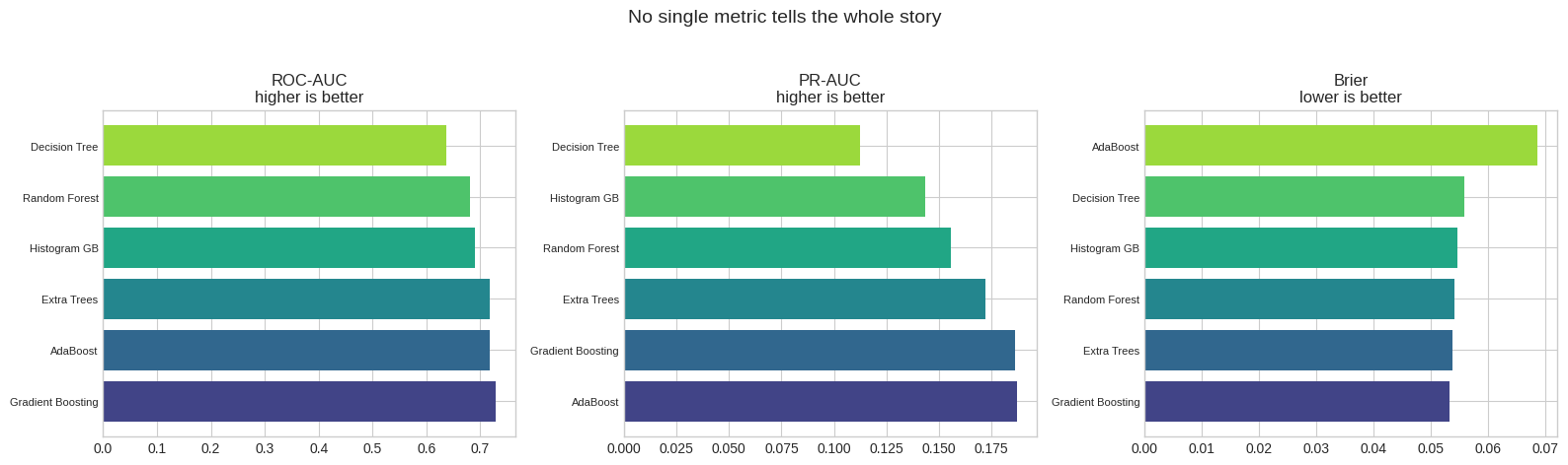
Three metrics, three different winners. Gradient Boosting leads on ROC-AUC at 0.7295, AdaBoost edges it on PR-AUC, Gradient Boosting takes Brier.
Meanwhile every model scores roughly 94% accuracy, including the one with an ROC-AUC of 0.637. At a 6% positive rate, accuracy is decoration.
Speed also splits from quality. Histogram Gradient Boosting fits in 0.29 seconds. Random Forest takes 4.25 seconds for a worse PR-AUC.
Bagging cuts variance, visibly
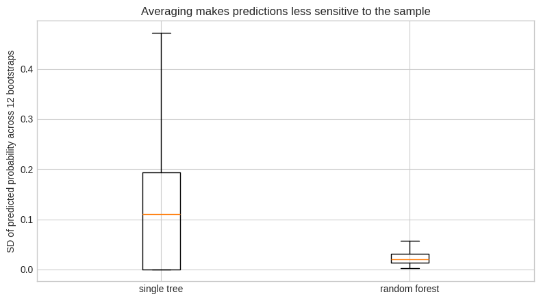
Twelve bootstrap resamples. A single deep tree moves with a mean prediction SD of 0.1175. A forest fit on the same resamples moves 0.0247.
That is the whole bagging argument in one number, and it is measured, not asserted.
Boosting needs a stopping rule
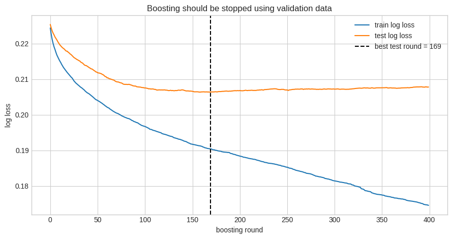
Train log loss keeps falling for all 400 rounds. Test log loss bottoms out at round 169 and then drifts back up.
The notebook is explicit that picking 169 from the test set is illustration only. In production that choice belongs to a validation fold.
Impurity importance rewards the noise column
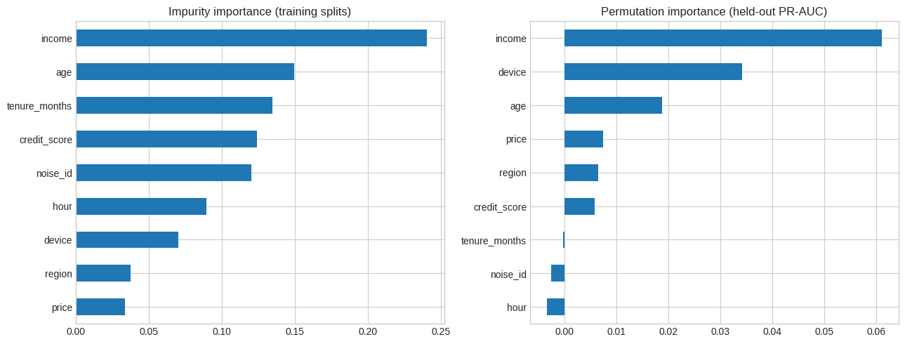
The planted useless ID column lands fifth of nine on mean decrease in impurity, at 0.1204. It offers thousands of candidate cut points, so the training splits reward it.
Permutation importance on held-out data gives it -0.0025. Breaking it makes the model slightly better.
This is the single most useful figure in the notebook if you have ever shipped an MDI bar chart to a stakeholder.
What the ranking is worth commercially
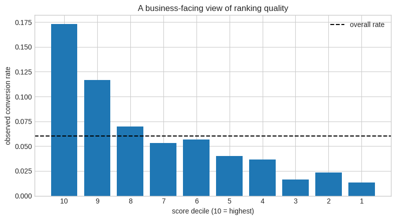
Top decile converts at 17.3%, which is 2.89 times the base rate. Bottom decile converts at 1.3%. A modest AUC still sorts the population well enough to be worth money.
Trees without a target
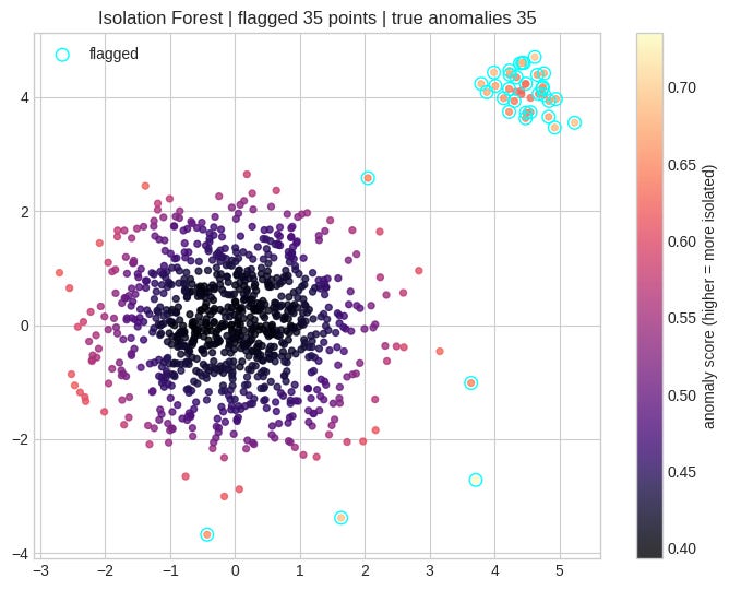
Isolation Forest partitions at random and calls the quickly isolated points anomalous. It recovers all 35 planted outliers here, plus a handful of legitimate tail points. Sparse is not the same as fraudulent.
Also in there
Native NaN routing in Histogram Gradient Boosting, tested on 297 test rows with a missing credit score and no imputer anywhere. A monotonic constraint forcing conversion to be non-increasing in price, which still reaches 0.7009 ROC-AUC. Partial dependence, with the warning that it is a model diagnostic and not a causal effect. A note on where XGBoost, LightGBM and CatBoost actually differ. A closing claim audit with verdicts.
Running it
Top to bottom, roughly two minutes on a laptop. Seeded, so your numbers should match the ones above.
Then break it on purpose. Push the positive rate to 1% and watch ROC-AUC and PR-AUC diverge. Corrupt 5% of the labels and see how badly AdaBoost handles it. Raise the cardinality of the noise column and watch MDI get worse. Remove the price constraint and look at what partial dependence says instead.
The best way to trust a model family is to find its failure mode yourself.